
Outcome Regression Estimator
The outcome regression estimator of the value of a fixed regime, \(d\), is defined as
\[ \widehat{\mathcal{V}}_{Q}(d) = n^{-1} \sum_{i=1}^{n} \left[ \sum_{a_{1} \in \mathcal{A}_{1}} Q_1(H_{1i},a_{1};\widehat{\beta}_{1}) ~ \text{I}\left\{d_{1}(H_{1i})=a_{1}\right\}\right], \]
where \(Q_{1}(h_{1},a_{1};\beta_{1})\) is a model for \(Q_{1}(h_{1},a_{1}) = E(Y|H_{1} = h_{1}, A_{1} = a_{1})\) and \(\widehat{\beta}_{1}\) is an estimator of \(\beta_{1}\).
For the previously defined \(\widehat{\mathcal{V}}_{Q}(d)\) for which the parameters of \(Q_{1}(h_{1}, a_{1};\beta_{1})\) are estimated using ordinary least squares (OLS), the \((1,1)\) component of the sandwich estimator for the variance is defined as
\[ \widehat{\Sigma}_{11} = A_{n} + (C_{n}^{\intercal}~D_{n}^{-1})~B_{n}~(C_{n}^{\intercal}~D_{n}^{-1})^{\intercal} , \]
where \(A_{n} = n^{-1} \sum_{i=1}^{n} A_{ni} A_{ni}\), \(B_{n} = n^{-1} \sum_{i=1}^{n} B_{ni} B_{ni}^{\intercal}\),
\[ A_{ni} = \left[ \sum_{a_{1} \in \mathcal{A}_{1}} Q_1(H_{1i},a_{1};\widehat{\beta}_{1}) ~ \text{I}\left\{d_{1}(H_{1i})=a_{1}\right\}\right] - \widehat{\mathcal{V}}_{Q}(d), \] and
\[ B_{ni} = \left\{Y_{i} - Q_{1}(H_{1i},A_{1i};\widehat{\beta}_{1})\right\} \frac{\partial Q_{1}(H_{1i},A_{1i};\widehat{\beta}_{1})}{\partial \beta_{1}}. \]
Terms \(C_{n}\) and \(D_{n}\) are the derivatives with respect to the parameters of the outcome regression model:
\[ C_{n} = n^{-1}\sum_{i=1}^{n}\frac{\partial A_{ni}}{\partial \beta_{1}} \quad \text{and} \quad D_{n} = n^{-1}\sum_{i=1}^{n} \frac{\partial B_{ni}}{\partial \beta_{1}^{\intercal}}. \]
Anticipating later methods, we break the implementation of the value estimator and the sandwich estimator of the variance into multiple functions, each function calculating a specific component. In addition, we reuse function
value_OR_se() : returns the value estimated using the outcome regression estimator and its standard error estimated using the sandwich variance estimator.value_OR_swv() : returns the outcome regression estimator component of the M-estimating equations and its derivatives, i.e., \(A_n\) and \(C^{\intercal}_n\) of the sandwich variance expression.value_OR() : returns the outcome regression estimator of the value of a fixed regime.swv_OLS() : returns the component of the M-estimating equation due to an ordinary least squares estimation of the parameters of a linear regression model and the inverse of the derivatives of that component, i.e., \(B_n\) and \(D^{-1}_n\) of the sandwich variance expression.
This implementation is not the most efficient implementation of the variance estimator. For example, the regression step is completed twice (once in
#------------------------------------------------------------------------------#
# outcome regression estimator for value of a fixed binary tx regime
#
# ASSUMPTIONS
#   tx is binary coded as {0,1}
#
# INPUTS
#    moOR : modeling object specifying outcome regression
#    data : data.frame containing baseline covariates and tx received
#           *** tx must be coded 0/1 ***
#       y : outcome of interest
#  txName : tx column in data (tx must be coded as 0/1)
#  regime : 0/1 vector containing recommended tx
#
# RETURNS
#  a list containing
#     fitOR : value object returned by outcome regression
#        EY : contribution to value from each tx
#  valueHat : estimated value
#------------------------------------------------------------------------------#
value_OR <- function(moOR, data, y, txName, regime) {

  #### Outcome Regression

  fitOR <- modelObj::fit(object = moOR, data = data, response = y)

  # estimated Q-function when all A=d
  data[,txName] <- regime
  Qd <- drop(x = modelObj::predict(object = fitOR, newdata = data))

  #### Value of regime

  EY <- array(data = 0.0, dim = 2L, dimnames = list(c("0","1")))
  EY[2L] <- mean(x = Qd*{regime == 1L})
  EY[1L] <- mean(x = Qd*{regime == 0L})

  value <- sum(EY)

  return( list("fitOR" = fitOR, "EY" = EY, "valueHat" = value) )
}
#------------------------------------------------------------------------------#
# value and standard error for the outcome regression estimator of the value
# of a fixed regime using the sandwich estimator of variance
#
# REQUIRES
# swv_OLS() and value_OR_swv()
#
# ASSUMPTIONS
# tx is binary coded as {0,1}
# moOR is a linear model with parameters to be estimated using OLS
#
# INPUTS
# moOR : modeling object specifying outcome regression
# *** must be a linear model ***
# data : data.frame containing covariates and tx
# *** tx must be coded 0/1 ***
# y : vector of outcome of interest
# txName : tx column in data (tx must be coded as 0/1)
# regime : 0/1 vector containing recommended tx
#
# RETURNS
# a list containing
# fitOR : value object returned by outcome regression
# EY : mean response for each tx
# valueHat : estimated value
# sigmaHat : estimated standard error
#------------------------------------------------------------------------------#
value_OR_se <- function(moOR, data, y, txName, regime) {
#### OLS components
OLS <- swv_OLS(mo = moOR, data = data, y = y)
#### estimator components
OR <- value_OR_swv(moOR = moOR,
data = data,
y = y,
regime = regime,
txName = txName)
#### 1,1 Component of Sandwich Estimator
# OLS contribution
temp <- OR$dMdB %*% OLS$invdM
sig11OLS <- temp %*% OLS$MM %*% t(x = temp)
sig11 <- drop(x = OR$MM + sig11OLS)
return( c(OR$value, "sigmaHat" = sqrt(x = sig11 / nrow(x = data))) )
}#------------------------------------------------------------------------------#
# component of sandwich estimator for outcome regression estimator of value of
# a fixed regime
#
# REQUIRES
# value_OR()
#
# ASSUMPTIONS
# outcome regression model is a linear model
# tx is binary coded as {0,1}
#
# INPUTS
# moOR : modeling object for outcome regression
# *** must be a linear model ***
# data : data.frame containing baseline covariates and tx
# *** tx must be coded 0/1 ***
# y : outcome of interest
# txName : tx column in data (tx must be coded as 0/1)
# regime : 0/1 vector containing recommended tx
#
# RETURNS
# a list containing
# value : list returned by value_OR()
# MM : M M^T matrix
# dMdB : matrix of derivatives of M wrt beta
#------------------------------------------------------------------------------#
value_OR_swv <- function(moOR, data, y, txName, regime) {
# estimate value
value <- value_OR(moOR = moOR,
data = data,
y = y,
regime = regime,
txName = txName)
# Q(H,d;betaHat)
data[,txName] <- regime
Qd <- drop(x = modelObj::predict(object = value$fit, newdata = data))
# derivative of Q(H,0;betaHat)
dQd <- stats::model.matrix(object = modelObj::model(object = moOR),
data = data)
# value component of M MT
mmt <- mean(x = {Qd - value$valueHat}^2)
# derivative of value component w.r.t. beta
dMdB <- colMeans(x = dQd)
return( list("value" = value, "MM" = mmt, "dMdB" = dMdB) )
}#------------------------------------------------------------------------------#
# components of the sandwich estimator for an ordinary least squares estimation
# of a linear regression model
#
# ASSUMPTIONS
# mo is a linear model with parameters to be estimated using OLS
#
# INPUTS
# mo : a modeling object specifying a regression step
# *** must be a linear model ***
# data : a data.frame containing covariates and tx
# y : a vector containing the outcome of interest
#
#
# RETURNS
# a list containing
# MM : M^T M component from OLS
# invdM : inverse of the matrix of derivatives of M wrt beta
#------------------------------------------------------------------------------#
swv_OLS <- function(mo, data, y) {
n <- nrow(x = data)
fit <- modelObj::fit(object = mo, data = data, response = y)
# Q(X,A;betaHat)
Qa <- drop(x = modelObj::predict(object = fit, newdata = data))
# derivative of Q(X,A;betaHat)
dQa <- stats::model.matrix(object = modelObj::model(object = mo),
data = data)
# number of parameters in model
p <- ncol(x = dQa)
# OLS component of M
mOLSi <- {y - Qa}*dQa
# OLS component of M MT
mmOLS <- sapply(X = 1L:n,
FUN = function(i){ mOLSi[i,] %o% mOLSi[i,] },
simplify = "array")
# derivative OLS component
dmOLS <- - sapply(X = 1L:n,
FUN = function(i){ dQa[i,] %o% dQa[i,] },
simplify = "array")
# sum over individuals
if (p == 1L) {
mmOLS <- mean(x = mmOLS)
dmOLS <- mean(x = dmOLS)
} else {
mmOLS <- rowMeans(x = mmOLS, dim = 2L)
dmOLS <- rowMeans(x = dmOLS, dim = 2L)
}
# invert derivative OLS component
invD <- solve(a = dmOLS)
return( list("MM" = mmOLS, "invdM" = invD) )
}It is now straightforward to estimate the value and the standard error for a variety of linear models. As was done in Chapter 2, we consider three outcome regression models selected to represent a range of model (mis)specification (see \(Q_{1}(h_{1},a_{1};\beta_{1})\) in sidebar for a review of the models and their basic diagnostics).
We also compare the estimated value under a variety of fixed regimes, \(d\). Each tab below illustrates the implementation for the respective fixed regime using only the correctly specified outcome regression model
\[ Q^{3}_{1}(h_{1},a_{1};\beta_{1}) = \beta_{10} + \beta_{11} \text{Ch} + \beta_{12} \text{K} + a_{1}~(\beta_{13} + \beta_{14} \text{Ch} + \beta_{15} \text{K}). \]
However, the estimated value and standard errors under all three outcome regression models are summarized at the end of each example.
We first consider static regime \(d\) characterized by rule \(d_{1}(h_{1}) \equiv 1\) for all \(h_{1} \in \mathcal{H}_{1}\). That is, all individuals are recommended to receive treatment \(A_{1} = 1\).
For \(Q^{3}_{1}(h_{1},a_{1};\beta_{1})\) the estimated value of this fixed regime and its standard error are obtained as follows:
q3 <- modelObj::buildModelObj(model = ~ (Ch + K)*A,
                              solver.method = 'lm',
                              predict.method = 'predict.lm')
regime <- rep(x = 1L, times = nrow(x = dataSBP))value_OR_se(moOR = q3, data = dataSBP, y = y, regime = regime, txName = 'A')$fitOR
Call:
lm(formula = YinternalY ~ Ch + K + A + Ch:A + K:A, data = data)
Coefficients:
(Intercept) Ch K A Ch:A
-15.6048 -0.2035 12.2849 -61.0979 0.5048
K:A
-6.6099
$EY
0 1
0.00000 10.24417
$valueHat
[1] 10.24417
$sigmaHat
[1] 0.4464732We see that for static regime \(d\) defined by rule \(d_{1}(H_{1}) \equiv 1\) for all \(h_{1}\), \(\widehat{\mathcal{V}}_{Q}(d) = 10.24 (0.45)\) mmHg, which is the sample mean of \(Q_{1}^{3}(h_{1},1;\widehat{\beta}_{1})\), $EY. Estimates under models \(Q^{1}_{1}(h_{1},a_{1};\beta_{1})\) and \(Q^{2}_{1}(h_{1},a_{1};\beta_{1})\) are similarly obtained.
In the table below, we see that the estimated value of regime \(d_{1}(H_{1}) \equiv 1\) under each of the three models considered ranges from 10.21 mmHg to 14.26 mmHg and that the results under models \(Q^{2}_{1}(h_{1},a_{1};\beta_{1})\) and \(Q^{3}_{1}(h_{1},a_{1};\beta_{1})\) are similar.
| (mmHg) | \(Q^{1}_{1}(h_{1},a_{1};\beta_{1})\) | \(Q^{2}_{1}(h_{1},a_{1};\beta_{1})\) | \(Q^{3}_{1}(h_{1},a_{1};\beta_{1})\) |
| \(\widehat{\mathcal{V}}_{Q}(d)\) | 14.26 (0.62) | 10.21 (0.45) | 10.24 (0.45) |
Next we consider static regime \(d\) characterized by rule \(d_{1}(h_{1}) \equiv 0\) for all \(h_{1} \in \mathcal{H}_{1}\). That is, all individuals are recommended to receive treatment \(A_{1} = 0\).
For \(Q^{3}_{1}(h_{1},a_{1};\beta_{1})\) the estimated value of this fixed regime and its standard error are obtained as follows:
q3 <- modelObj::buildModelObj(model = ~ (Ch + K)*A,
                              solver.method = 'lm',
                              predict.method = 'predict.lm')
regime <- rep(x = 0L, times = nrow(x = dataSBP))value_OR_se(moOR = q3, data = dataSBP, y = y, regime = regime, txName = 'A')$fitOR
Call:
lm(formula = YinternalY ~ Ch + K + A + Ch:A + K:A, data = data)
Coefficients:
(Intercept) Ch K A Ch:A
-15.6048 -0.2035 12.2849 -61.0979 0.5048
K:A
-6.6099
$EY
0 1
-6.458372 0.000000
$valueHat
[1] -6.458372
$sigmaHat
[1] 0.3361539We see that for static regime \(d\) defined by the rule \(d_{1}(H_{1}) \equiv 0\) for all \(h_{1}\), \(\widehat{\mathcal{V}}(d) = -6.46 (0.34)\) mmHg, which is the sample mean of \(Q_{1}^{3}(h_{1},0;\widehat{\beta}_{1})\), $EY. Estimates under models \(Q^{1}_{1}(h_{1},a_{1};\beta_{1})\) and \(Q^{2}_{1}(h_{1},a_{1};\beta_{1})\) are similarly obtained.
In the table below, we see that the estimated value of regime \(d_{1}(H_{1}) \equiv 1\) under each of the three models considered ranges from -6.46 mmHg to -4.18 mmHg and that the results under models \(Q^{2}_{1}(h_{1},a_{1};\beta_{1})\) and \(Q^{3}_{1}(h_{1},a_{1};\beta_{1})\) are similar.
| (mmHg) | \(Q^{1}_{1}(h_{1},a_{1};\beta_{1})\) | \(Q^{2}_{1}(h_{1},a_{1};\beta_{1})\) | \(Q^{3}_{1}(h_{1},a_{1};\beta_{1})\) |
| \(\widehat{\mathcal{V}}_{Q}(d)\) | -4.18 (0.43) | -6.43 (0.36) | -6.46 (0.34) |
Next, we consider a simple regime that depends on covariates, say \(d\) is characterized by rule
\[ d_{1}(H_{1}) = \text{I}(\text{Ch} > 100~ \text{mg/dl}). \]
Under this regime, individuals with cholesterol measurements greater than 100 mg/dl receive our fictitious medication; all others do not. For \(Q^{3}_{1}(h_{1},a_{1};\beta_{1})\) the estimated value of this fixed regime and its standard error are obtained as follows:
q3 <- modelObj::buildModelObj(model = ~ (Ch + K)*A,
                              solver.method = 'lm',
                              predict.method = 'predict.lm')
regime <- as.integer(x = {dataSBP$Ch > 100})value_OR_se(moOR = q3, data = dataSBP, y = y, regime = regime, txName = 'A')$fitOR
Call:
lm(formula = YinternalY ~ Ch + K + A + Ch:A + K:A, data = data)
Coefficients:
(Intercept) Ch K A Ch:A
-15.6048 -0.2035 12.2849 -61.0979 0.5048
K:A
-6.6099
$EY
0 1
0.03791634 10.32527006
$valueHat
[1] 10.36319
$sigmaHat
[1] 0.4415434We see that for static regime \(d\) defined by the rule \(d_{1}(H_{1}) = \text{I}(\text{Ch} > 100~ \text{mg/dl})\) is \(\widehat{\mathcal{V}}(d) = 10.36 (0.44)\) mmHg. Not unexpectedly, this result is very similar to that obtained for \(d\) defined by the rule \(d_{1}(H_{1}) \equiv 1\); most individuals in our data set have cholesterol levels above 100 mg/dl and thus are recommended to treatment \(A_{1} = 1\). Estimates under models \(Q^{1}_{1}(h_{1},a_{1};\beta_{1})\) and \(Q^{2}_{1}(h_{1},a_{1};\beta_{1})\) are similarly obtained.
In the table below, we see that the estimated value of regime \(d_{1}(H_{1}) \equiv 1\) under each of the three models considered ranges from 10.34 mmHg to 14.2 mmHg and that the results under models \(Q^{2}_{1}(h_{1},a_{1};\beta_{1})\) and \(Q^{3}_{1}(h_{1},a_{1};\beta_{1})\) are similar.
| (mmHg) | \(Q^{1}_{1}(h_{1},a_{1};\beta_{1})\) | \(Q^{2}_{1}(h_{1},a_{1};\beta_{1})\) | \(Q^{3}_{1}(h_{1},a_{1};\beta_{1})\) |
| \(\widehat{\mathcal{V}}_{Q}(d)\) | 14.20 (0.62) | 10.34 (0.45) | 10.36 (0.44) |
A more interesting question might be “how does \(\widehat{\mathcal{V}}_{Q}(d)\) depend on the constant cutoff, \(c\)?” To determine this, we can estimate the value over a grid of \(c\) values that span the range of measured cholesterol levels 83 mg/dl \(\le\) Ch \(\le\) 333 mg/dl. For example,
q3 <- modelObj::buildModelObj(model = ~ (Ch + K)*A,
                              solver.method = 'lm',
                              predict.method = 'predict.lm')
# obtain a grid of Ch values spanning range
cValues <- seq(from = floor(x = min(x = dataSBP$Ch)),
to = ceiling(x = max(x = dataSBP$Ch)),
length.out = 100L)
regimes <- sapply(X = cValues, FUN = function(x,y){{y > x}*1L}, y = dataSBP$Ch)OR3c <- apply(X = regimes,
MARGIN = 2L,
FUN = function(x, moOR, data, y) {
temp <- value_OR_se(moOR = moOR,
data = data,
y = y,
regime = x,
txName = 'A')
return( c("valueHat" = temp$valueHat,
"sigmaHat" = temp$sigmaHat) )
},
moOR = q3,
data = dataSBP,
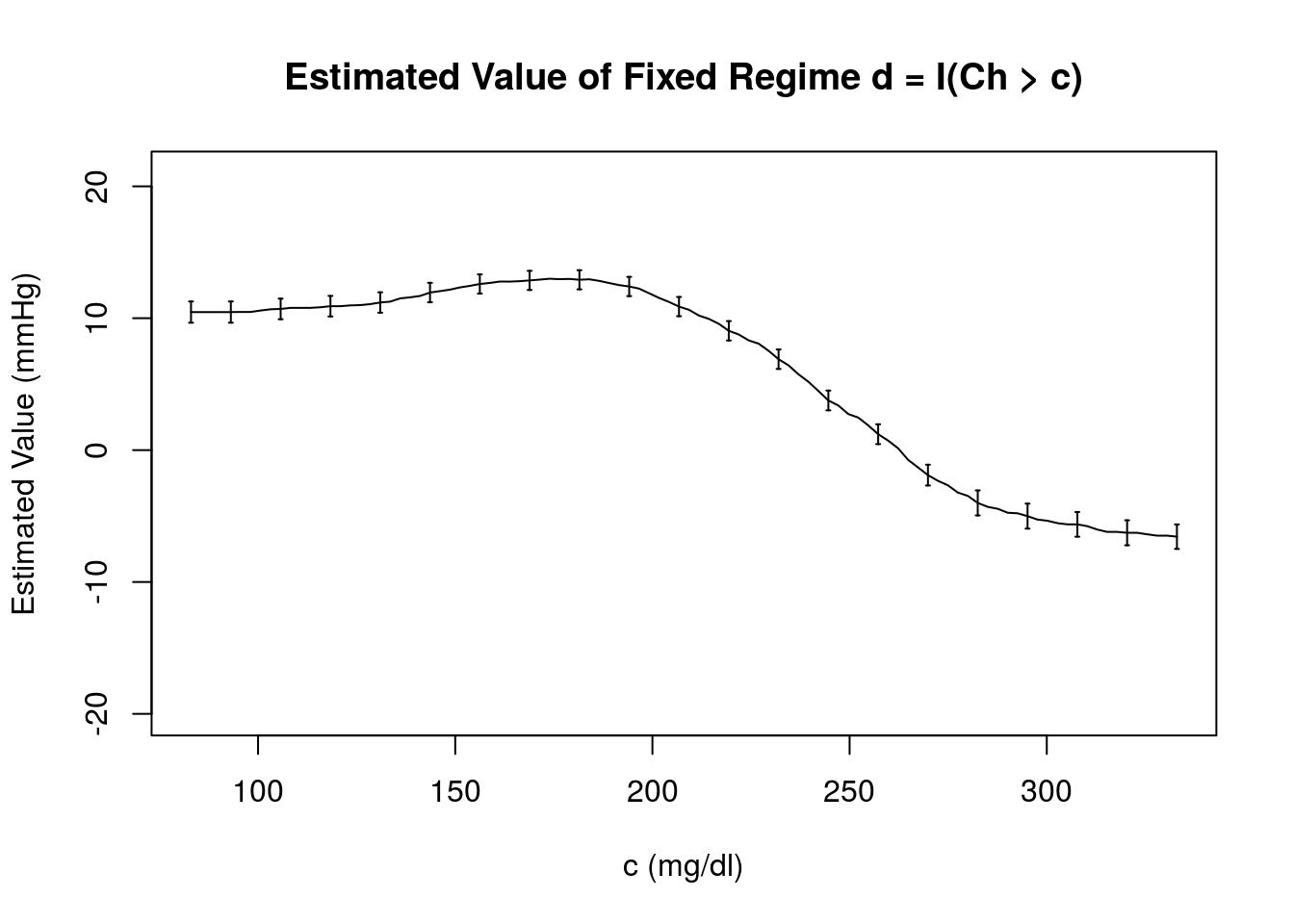
y = y)Below, we plot \(\widehat{\mathcal{V}}_{Q}(d)\) as a function of \(c\)

The structure seen in this plot is indicative of the fact that \(Q^{3}_{1}(h_{1},a_{1};\beta_{1})\) includes Ch. There is a clear maximum estimated value under this model, \(\widehat{\mathcal{V}}_{Q}(d) = 13.18\) mmHg, which occurs near \(c = 176.43\) mg/dl. In the comparison below, we see that this result is model dependent.

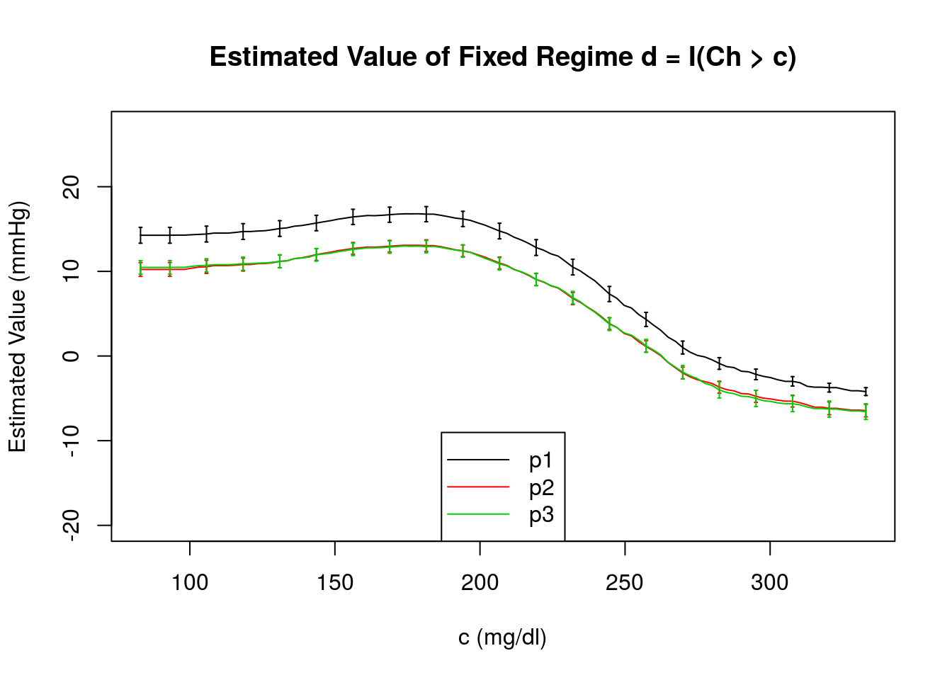
In this figure, we compare the estimated value of regime \(d = \{d_{1}(H_{1})\} = \text{I}(\text{Ch}>c)\) obtained using the regression estimator and its estimated standard error obtained under each of the outcome regression models under consideration. We see that for \(Q^{1}_{1}(h_{1},a_{1};\beta_{1})\), the value smoothly transitions from a maximum when all individuals have \(\text{Ch} >\) 83 mg/dl to the minimum when all individuals have \(\text{Ch} <\) 333 mg/dl; this smooth structure is indicative of the normal distribution of the data generating model for Ch and the absence of covariate Ch in the outcome model. For the incomplete and true models, which do contain Ch, the values and standard errors obtained are very similar with a maximum near Ch = \(c = 176.43\) mg/dl. Note that we include the estimated standard errors for only a subset of \(c\).
IPW Estimator
The inverse probability weighted (IPW) estimator of the value of fixed regime \(d\) is defined as
\[ \widehat{\mathcal{V}}_{IPW}(d) = n^{-1} \sum_{i=1}^{n} \frac{\mathcal{C}_{d,i}Y_{i}}{\pi_{d,1}(H_{1i};\widehat{\gamma}_{1})}, \] where
\[ \mathcal{C}_{d} = \text{I}\{A_{1} = d_{1}(H_{1})\} \] is the indicator that the treatment option actually received coincides with that dictated by \(d\).
The propensity for receiving treatment consistent with regime \(d\) given an individual’s history is \(\pi_{d,1}(H_{1}) = P(\mathcal{C}_{d} = 1|H_{1})\). It is straightforward to deduce that
\[ \pi_{d,1}(H_{1}) = \pi_{1}(H_{1}) ~ \text{I}\{d_{1}(H_{1}) = 1\} + \{1-\pi_{1}(H_{1})\} ~ \text{I}\{d_{1}(H_{1}) = 0\}, \] which can be estimated by positing a model \(\pi_{1}(H_{1};\gamma_{1})\) for \(\pi_{1}(H_{1}) = P(A_{1} = 1|H_{1})\). Thus
\[ \pi_{d,1}(H_{1}; \gamma_{1}) = \pi_{1}(H_{1}; \gamma_{1}) ~ \text{I}\{d_{1}(H_{1}) = 1\} + \{1-\pi_{1}(H_{1}; \gamma_{1})\} ~ \text{I}\{d_{1}(H_{1}) = 0\}, \] and \(\widehat{\gamma}_{1}\) is a suitable estimator for \(\gamma_{1}\).
For the previously defined \(\widehat{\mathcal{V}}_{IPW}(d)\) for which \(\pi_{1}(h_{1};\gamma_{1})\) is a logistic regression model with parameters estimated using maximum likelihood, the \((1,1)\) component of the sandwich estimator for the variance is defined as
\[ \widehat{\Sigma}_{11} = A_{n} + (C_{n}^{\intercal}~D_{n}^{-1})~B_{n}~(C_{n}^{\intercal}~D_{n}^{-1})^{\intercal} , \]
where \(A_{n} = n^{-1} \sum_{i=1}^{n} A_{ni} A_{ni}\) and \(B_{n} = n^{-1} \sum_{i=1}^{n} B_{ni} B_{ni}^{\intercal}\)
\[ A_{ni} = \frac{C_{d,i}~Y_i}{\pi_{d,1}(H_{1i};\widehat{\gamma}_{1})} - \widehat{\mathcal{V}}_{IPW}(d), \] and \[ B_{ni} = \frac{ A_{1i} - \pi_{1}(H_{1i};\widehat{\gamma}_{1})}{\pi_{1}(H_{1i}; \widehat{\gamma}_{1})\{1-\pi_{1}(H_{1i}; \widehat{\gamma}_{1})\}} \frac{\partial \pi_{1}(H_{1i}; \widehat{\gamma}_{1})}{\partial \gamma_{1}}. \]
Terms \(C_{n}\) and \(D_{n}\) are the derivatives with respect to the parameters of the propensity score model:
\[ C_{n} = n^{-1}\sum_{i=1}^{n}\frac{\partial A_{ni}}{\partial \gamma_{1}} \quad \text{and} \quad D_{n} = n^{-1}\sum_{i=1}^{n} \frac{\partial B_{ni}}{\partial \gamma_{1}^{\intercal}}. \]
Anticipating later methods, we break the implementation of the value estimator and the sandwich estimator of the variance into multiple functions, each function calculating a specific component. In addition, we reuse function
value_IPW_se() : returns the value estimated using the inverse probability weighted estimator and its standard error estimated using the sandwich variance estimator.value_IPW_swv() : returns the inverse probability weighted estimator component of the M-estimating equations and its derivatives, i.e., \(A_n\) and \(C^{\intercal}_n\) of the sandwich variance expression.value_IPW() : returns the inverse probability weighted estimator of the value of a fixed regime.swv_ML() : returns the component of the M-estimating equation due to a maximum likelihood estimation of the parameters of a logistic regression model and the inverse of the derivatives of that component, i.e., \(B_n\) and \(D^{-1}_n\) of the sandwich variance expression.
This implementation is not the most efficient implementation of the variance estimator. For example, the regression step is completed twice (once in
#------------------------------------------------------------------------------#
# IPW estimator for value of a fixed binary tx regime
#
# ASSUMPTIONS
#   tx is binary coded as {0,1}
#
# INPUTS
#    moPS : modeling object specifying propensity score regression
#    data : data.frame containing baseline covariates and tx
#           *** tx must be coded 0/1 ***
#       y : outcome of interest
#  txName : tx column in data (tx must be coded as 0/1)
#  regime : 0/1 vector containing recommended tx
#
# RETURNS
#  a list containing
#     fitPS : value object returned by propensity score regression
#        EY : sample average outcome for each tx
#  valueHat : estimated value
#------------------------------------------------------------------------------#
value_IPW <- function(moPS, data, y, txName, regime) {

  #### Propensity Score Regression
  fitPS <- modelObj::fit(object = moPS, data = data, response = data[,txName])

  # estimate propensity score
  p1 <- modelObj::predict(object = fitPS, newdata = data)
  if (is.matrix(x = p1)) p1 <- p1[,ncol(x = p1), drop = TRUE]

  #### Value Estimate

  EY <- array(data = 0.0, dim = 2L, dimnames = list(c("0","1")))
  sub1 <- {regime == data[,txName]} & {data[,txName] == 1L}
  sub0 <- {regime == data[,txName]} & {data[,txName] == 0L}
  EY[2L] <- mean(x = sub1 * y / p1)
  EY[1L] <- mean(x = sub0 * y / {1.0 - p1})

  value <- sum(EY)

  return( list("fitPS" = fitPS, "EY" = EY, "valueHat" = value) )
}
#------------------------------------------------------------------------------#
# value and standard error for the IPW estimator of the value of a fixed regime
# using the sandwich estimator of variance
#
# REQUIRES
# swv_ML() and value_IPW_swv()
#
# ASSUMPTIONS
# tx is binary coded as {0,1}
# moPS is a logistic model
#
# INPUTS
# moPS : modeling object specifying propensity score regression
# *** must be a logistic model ***
# data : data.frame containing covariates and tx
# *** tx must be coded 0/1 ***
# y : vector of outcome of interest
# txName : tx column in data (tx must be coded as 0/1)
# regime : 0/1 vector containing recommended tx
#
# RETURNS
# a list containing
# fitPS : modelObjFit object for propensity score regression
# EY : sample average outcome for each tx
# valueHat : estimated value
# sigmaHat : estimated standard error
#------------------------------------------------------------------------------#
value_IPW_se <- function(moPS, data, y, txName, regime) {
# obtain ML components
ML <- swv_ML(mo = moPS, data = data, y = data[,txName])
# obtain IPW value components
IPW <- value_IPW_swv(moPS = moPS,
data = data,
y = y,
regime = regime,
txName = txName)
# calculate 1,1 component
temp <- IPW$dMdG %*% ML$invdM
sig11 <- drop(x = IPW$MM + temp %*% ML$MM %*% t(x = temp))
return( c(IPW$value, "sigmaHat" = sqrt(x = sig11/ nrow(x = data))) )
}#------------------------------------------------------------------------------#
# component of sandwich estimator for IPW estimator of value of a fixed regime
#
# REQUIRES
# value_IPW()
#
# ASSUMPTIONS
# propensity score model is a logistic model
# tx is binary coded as {0,1}
#
# INPUTS
# moPS : modeling object for propensity score regression
# *** must be a logistic model ***
# data : data.frame containing baseline covariates and tx
# *** tx must be coded 0/1 ***
# y : outcome of interest
# txName : tx column in data (tx must be coded as 0/1)
# regime : 0/1 vector containing recommended tx
#
# RETURNS
# a list containing
# value : list returned by value_IPW()
# MM : M M^T matrix
# dMdG : matrix of derivatives of M wrt gamma
#------------------------------------------------------------------------------#
value_IPW_swv <- function(moPS, data, y, txName, regime) {
# estimate value
value <- value_IPW(moPS = moPS,
data = data,
y = y,
regime = regime,
txName = txName)
# pi(x; gamma)
p1 <- modelObj::predict(object = value$fitPS, newdata = data)
if (is.matrix(x = p1)) p1 <- p1[,ncol(x = p1), drop = TRUE]
# model.matrix for propensity model
piMM <- stats::model.matrix(object = modelObj::model(object = moPS),
data = data)
# propensity for receiving recommended tx
pid <- p1*{regime == 1L} + {1.0-p1}*{regime == 0L}
# indicator of tx received = regime
Cd <- regime == data[,txName]
# value component of M MT
mmValue <- mean(x = {Cd * y / pid - value$valueHat}^2)
# derivative w.r.t. gamma
dMdG <- colMeans(x = Cd * y / pid * (-regime + p1) * piMM)
return( list("value" = value, "MM" = mmValue, "dMdG" = dMdG) )
}#------------------------------------------------------------------------------#
# components of the sandwich estimator for a maximum likelihood estimation of
# a logistic regression model
#
# ASSUMPTIONS
# mo is a logistic model with parameters to be estimated using ML
#
# INPUTS
# mo : a modeling object specifying a regression step
# *** must be a logistic model ***
# data : a data.frame containing covariates and tx
# y : a vector containing the binary outcome of interest
#
#
# RETURNS
# a list containing
# MM : M^T M component from ML
# invdM : inverse of the matrix of derivatives of M wrt gamma
#------------------------------------------------------------------------------#
swv_ML <- function(mo, data, y) {
# regression step
fit <- modelObj::fit(object = mo, data = data, response = y)
# yHat
p1 <- modelObj::predict(object = fit, newdata = data)
if (is.matrix(x = p1)) p1 <- p1[,ncol(x = p1), drop = TRUE]
# model.matrix for model
piMM <- stats::model.matrix(object = modelObj::model(object = mo),
data = data)
n <- nrow(x = piMM)
p <- ncol(x = piMM)
# ML M-estimator component
mMLi <- {y - p1} * piMM
# ML component of M MT
mmML <- sapply(X = 1L:n,
FUN = function(i){ mMLi[i,] %o% mMLi[i,] },
simplify = "array")
# derivative of ML component
dFun <- function(i){
- piMM[i,] %o% piMM[i,] * p1[i] * {1.0 - p1[i]}
}
dmML <- sapply(X = 1L:n, FUN = dFun, simplify = "array")
if( p == 1L ) {
mmML <- mean(x = mmML)
dmML <- mean(x = dmML)
} else {
mmML <- rowMeans(x = mmML, dim = 2L)
dmML <- rowMeans(x = dmML, dim = 2L)
}
# invert derivative ML component
invD <- solve(a = dmML)
return( list("MM" = mmML, "invdM" = invD) )
}It is now straightforward to estimate the value and the standard error for a variety of logistic regression models. As was done in Chapter 2, we consider three propensity score models selected to represent a range of model (mis)specification (see \(\pi_{1}(h_{1};\gamma_{1})\) in menu to the left for a review of the models and their basic diagnostics).
As was done for the outcome regression estimator, we compare the estimated value under a variety of fixed regimes. Each tab below illustrates how to define the fixed regime under consideration and complete an analysis using the correctly specified propensity score model
\[ \pi^{3}_{1}(h_{1};\gamma_{1}) = \frac{\exp(\gamma_{10} + \gamma_{11}~\text{SBP0} + \gamma_{12}~\text{Ch})}{1+\exp(\gamma_{10} + \gamma_{11}~\text{SBP0}+ \gamma_{12}~\text{Ch})}. \]
The estimated value and standard errors under all three models are summarized at the end of each example.
First we consider static regime \(d\) characterized by rule \(d_{1}(h_{1}) \equiv 1\) for all \(h_{1} \in \mathcal{H}_{1}\). That is, all individuals are recommended to receive treatment \(A_{1} = 1\).
For \(\pi^{3}_{1}(h_{1};\gamma_{1})\) the estimated value of this fixed regime and its standard error are obtained as follows:
p3 <- modelObj::buildModelObj(model = ~ SBP0 + Ch,
                              solver.method = 'glm',
                              solver.args = list(family='binomial'),
                              predict.method = 'predict.glm',
                              predict.args = list(type='response'))
regime <- rep(x = 1L, times = nrow(x = dataSBP))value_IPW_se(moPS = p3, data = dataSBP, y = y, regime = regime, txName = 'A')$fitPS
Call: glm(formula = YinternalY ~ SBP0 + Ch, family = "binomial", data = data)
Coefficients:
(Intercept) SBP0 Ch
-15.94153 0.07669 0.01589
Degrees of Freedom: 999 Total (i.e. Null); 997 Residual
Null Deviance: 1378
Residual Deviance: 1162 AIC: 1168
$EY
0 1
0.00000 10.44592
$valueHat
[1] 10.44592
$sigmaHat
[1] 0.8041447We see that the inverse probability weighted estimator of the value under \(d_{1}(H_{1}) \equiv 1\) is 10.45 (0.80) mmHg. Estimates under models \(\pi^{1}_{1}(h_{1};\gamma_{1})\) and \(\pi^{2}_{1}(h_{1};\gamma_{1})\) are similarly obtained.
In the table below, we see that the estimated value of regime \(d = \{d_{1}(h_{1}) \equiv 1\}\) under each of the models considered ranges from 10.21 mmHg to 14.23 mmHg and that the results under models \(\pi^{2}_{1}(h_{1};\gamma_{1})\) and \(\pi^{3}_{1}(h_{1};\gamma_{1})\) are similar.
| (mmHg) | \(\pi^{1}_{1}(h_{1};\gamma_{1})\) | \(\pi^{2}_{1}(h_{1};\gamma_{1})\) | \(\pi^{3}_{1}(h_{1};\gamma_{1})\) |
| \(\widehat{\mathcal{V}}_{IPW}(d)\) | 14.23 (0.94) | 10.21 (0.82) | 10.45 (0.80) |
Next we consider is static regime \(d\) characterized by rule \(d_{1}(h_{1}) \equiv 0\) for all \(h_{1} \in \mathcal{H}_{1}\). That is, all individuals are recommended to receive treatment \(A_{1} = 0\).
For \(\pi^{3}_{1}(h_{1};\gamma_{1})\) the estimated value of this fixed regime and its standard error are obtained as follows:
p3 <- modelObj::buildModelObj(model = ~ SBP0 + Ch,
                              solver.method = 'glm',
                              solver.args = list(family='binomial'),
                              predict.method = 'predict.glm',
                              predict.args = list(type='response'))
regime <- rep(x = 0L, times = nrow(x = dataSBP))value_IPW_se(moPS = p3, data = dataSBP, y = y, regime = regime, txName = 'A')$fitPS
Call: glm(formula = YinternalY ~ SBP0 + Ch, family = "binomial", data = data)
Coefficients:
(Intercept) SBP0 Ch
-15.94153 0.07669 0.01589
Degrees of Freedom: 999 Total (i.e. Null); 997 Residual
Null Deviance: 1378
Residual Deviance: 1162 AIC: 1168
$EY
0 1
-6.562869 0.000000
$valueHat
[1] -6.562869
$sigmaHat
[1] 0.9283407We see that the estimated value is -6.56 (0.93) mmHg.
In the table below, we see that the estimated value of regime \(d = \{d_{1}(h_{1}) \equiv 0\}\) under each of the models considered ranges from -6.56 mmHg to -4.20 mmHg and that again the results under models \(\pi^{2}_{1}(h_{1};\gamma_{1})\) and \(\pi^{3}_{1}(h_{1};\gamma_{1})\) are similar.
| (mmHg) | \(\pi^{1}_{1}(h_{1};\gamma_{1})\) | \(\pi^{2}_{1}(h_{1};\gamma_{1})\) | \(\pi^{3}_{1}(h_{1};\gamma_{1})\) |
| \(\widehat{\mathcal{V}}_{IPW}(d)\) | -4.20 (0.47) | -6.45 (0.74) | -6.56 (0.93) |
Finally, we consider a simple regime that depends on covariates, \[ d_{1}(H_{1}) = \text{I}(\text{Ch} > c). \]
Under this regime, individuals with cholesterol measurements greater than c (83 mg/dl \(\le\) c \(\le\) 333 mg/dl) receive our fictitious medication; all others do not. For \(Q^{3}_{1}(h_{1},a_{1};\beta_{1})\) the estimated value of this fixed regime and its standard error are obtained as follows:
p3 <- modelObj::buildModelObj(model = ~ SBP0 + Ch,
                              solver.method = 'glm',
                              solver.args = list(family='binomial'),
                              predict.method = 'predict.glm',
                              predict.args = list(type='response'))
# obtain a grid of Ch values spanning range
cValues <- seq(from = floor(x = min(x = dataSBP$Ch)),
to = ceiling(x = max(x = dataSBP$Ch)),
length.out = 100L)
regimes <- sapply(X = cValues, FUN = function(x,y){y > x}, y = dataSBP$Ch)IPW3c <- apply(X = regimes,
MARGIN = 2L,
FUN = function(x, moPS, data, y) {
temp <- value_IPW_se(moPS = moPS,
data = data,
y = y,
regime = x,
txName = 'A')
return( c("valueHat" = temp$valueHat,
"sigmaHat" = temp$sigmaHat) )
},
moPS = p3,
data = dataSBP,
y = y)
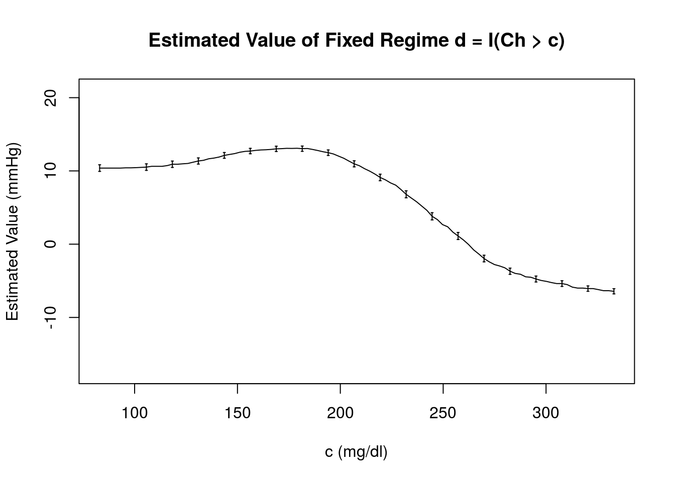
colnames(x = IPW3c) <- round(x = cValues, digits = 2)Below, we plot \(\widehat{\mathcal{V}}_{IPW}(d)\) as a function of \(c\)
The structure seen in this plot is similar to that obtained previously using the outcome regression estimator under the incomplete and true outcome regression models. There is a clear maximum estimated value under this model, \(\widehat{\mathcal{V}}_{IPW}(d) = 13\) mmHg, which occurs near \(c = 173.91\) mg/dl.
In this figure, we compare the estimated value of regime \(d = \{d_{1}(H_{1})\} = \text{I}(\text{Ch}>c)\) obtained using the IPW estimator, \(\widehat{\mathcal{V}}_{IPW}(d)\) and its standard error, \(\widehat{\sigma}_{11}\) obtained under each of the propensity score models under consideration. We see that the estimated value under \(\pi^{1}_{1}(h_{1};\gamma_{1})\) is consistently larger than that obtained under \(\pi^{2}_{1}(h_{1};\gamma_{1})\) and \(\pi^{3}_{1}(h_{1};\gamma_{1})\). Again, we include the standard errors for only a subset of \(c\) for clarity of presentation.
AIPW Estimator
The augmented inverse probability weighted estimator of the value of a fixed regime, \(d\), is defined as
\[ \widehat{\mathcal{V}}_{AIPW}(d) = n^{-1} \sum_{i=1}^{n} \left\{ \frac{\mathcal{C}_{d,i}Y_{i}}{\pi_{d,1}(H_{1i};\widehat{\gamma}_{1})} - \frac{\mathcal{C}_{d,i} - \pi_{d,1}(H_{1i};\widehat{\gamma}_{1})}{\pi_{d,1}(H_{1i};\widehat{\gamma}_{1})} \mathcal{Q}_{d,1}(H_{1i};\widehat{\beta}_{1}) \right\}, \]
where
\[ \mathcal{C}_{d} = \text{I}\{A_{1} = d_{1}(H_{1})\}, \] is the indicator that the treatment option actually received coincides with that dictated by \(d\).
The propensity for receiving treatment consistent with regime \(d\) given an individual’s history is \(\pi_{d,1}(H_{1}) = P(\mathcal{C}_{d} = 1|H_{1})\). It is straightforward to deduce that,
\[ \pi_{d,1}(H_{1}) = \pi_{1}(H_{1}) ~ \text{I}\{d_{1}(H_{1}) = 1\} + \{1-\pi_{1}(H_{1})\} ~ \text{I}\{d_{1}(H_{1}) = 0\}, \] which can be estimated by positing a model \(\pi_{1}(H_{1};\gamma_{1})\) for \(\pi_{1}(H_{1}) = P(A_{1} = 1|H_{1})\). Thus
\[ \pi_{d,1}(H_{1}; \gamma_{1}) = \pi_{1}(H_{1}; \gamma_{1}) ~ \text{I}\{d_{1}(H_{1}) = 1\} + \{1-\pi_{1}(H_{1}; \gamma_{1})\} ~ \text{I}\{d_{1}(H_{1}) = 0\}, \] and \(\widehat{\gamma}_{1}\) is a suitable estimator for \(\gamma_{1}\).
Finally, \[ \mathcal{Q}_{d,1} (H_{1}; \beta)= Q_{1}(H_{1},1;\beta)~\text{I}\{d_{1}(H_{1})=1\} +Q_{1}(H_{1},0;\beta)~ \text{I}\{d_{1}(H_{1})=0\}, \] where \(Q_{1}(h_{1},a_{1};\beta)\) is a model for \(Q_{1}(h_{1},a_{1}) = E(Y|H_{1} = h_{1}, A_{1} = a_{1})\) and \(\widehat{\beta}_{1}\) is a suitable estimator for \(\beta_{1}\).
For the previously defined \(\widehat{\mathcal{V}}_{AIPW}(d)\) for which \(\pi_{1}(h_{1};\gamma_{1})\) is a logistic regression model with parameters estimated using maximum likelihood and \(Q_{1}(h_{1},a_{1};\beta_{1})\) is a linear regression model with parameters estimated using ordinary least squares, the \((1,1)\) component of the sandwich estimator for the variance is defined as
\[ \widehat{\Sigma}_{11} =A_{n} + ( D_{n}^{\intercal}~E_{n}^{-1})~B_{n}~( D_{n}^{\intercal}~E_{n}^{-1})^{T} + ( G_{n}^{\intercal}~J_{n}^{-1})~C_{n}~( G_{n}^{\intercal}~J_{n}^{-1})^{T}, \]
where \(A_{n} = n^{-1} \sum_{i=1}^{n} A_{ni} A_{ni}^{\intercal}\), \(B_{n} = n^{-1} \sum_{i=1}^{n} B_{ni} B_{ni}^{\intercal}\), \(C_{n} = n^{-1} \sum_{i=1}^{n} C_{ni} C_{ni}^{\intercal}\), and
\[ \begin{aligned} A_{ni} &= \frac{\mathcal{C}_{d,i} Y_{i}}{\pi_{d,1}(H_{1i};\widehat{\gamma}_{1})} - \frac{\mathcal{C}_{d,i} - \pi_{d,1}(H_{1i};\widehat{\gamma}_{1})}{\pi_{d,1}(H_{1i};\widehat{\gamma}_{1})} \mathcal{Q}_{d,1}(H_{1i};\widehat{\beta}_{1}) - \widehat{\mathcal{V}}_{AIPW}(d), \\~\\ B_{ni} &= \left\{Y_{i} - Q_{1}(H_{1i},A_{1i};\widehat{\beta}_{1})\right\} \frac{\partial Q_{1}(H_{1i},A_{1i};\widehat{\beta}_{1})}{\partial \beta_{1}}, \quad \text{and}\\~\\ C_{ni} &= \frac{ A_{1i} - \pi_{1}(H_{1i};\widehat{\gamma}_{1})}{\pi_{1}(H_{1i};\widehat{\gamma}_{1})\{1-\pi_{1}(H_{1i};\widehat{\gamma}_{1})\}} \frac{\partial \pi_{1}(H_{1i};\widehat{\gamma}_{1})}{\partial \gamma_{1}}. \end{aligned} \]
Terms \(D_{n}\) and \(E_{n}\) are the non-zero derivatives of \(A_{ni}, B_{ni}, C_{ni}\) with respect to the parameters of the outcome regression model:
\[ D_n = n^{-1}\sum_{i=1}^{n}\frac{\partial A_{ni}}{\partial {\beta}_{1}} \quad \text{and} \quad E_{n} = n^{-1}\sum_{i=1}^{n}\frac{\partial B_{ni}}{\partial {\beta}^{\intercal}_{1}}. \]
And, terms \(G_{n}\) and \(J_{n}\) are the non-zero derivatives of \(A_{ni}, B_{ni}, C_{ni}\) with respect to the parameters of the propensity score model:
\[ G_{n} = n^{-1}\sum_{i=1}^{n}\frac{\partial A_{ni}}{\partial {\gamma}_{1}} \quad \text{and} \quad J_{n} = n^{-1} \sum_{i=1}^{n} \frac{\partial C_{ni}}{\partial {\gamma}^{\intercal}_{1}}. \]
As we have done previously, we break the implementation of the value estimator and the sandwich estimator of the variance into multiple functions, each function calculating a specific component. This structure allows us to reuse functions
value_AIPW_se() : returns the value estimated using the augmented inverse probability weighted estimator and its standard error estimated using the sandwich variance estimator.value_AIPW_swv() : returns the augmented inverse probability weighted estimator component of the M-estimating equations and its derivatives, i.e., \(A_{n}\), \(D_{n}^{\intercal}\), and \(G_{n}^{\intercal}\) of the sandwich variance expression.value_AIPW() : returns the augmented inverse probability weighted estimator of the value of a fixed regime.swv_OLS() : returns the component of the M-estimating equation due to an ordinary least squares estimation of the parameters of a linear regression model and the inverse of the derivatives of that component, i.e., \(B_n\) and \(E^{-1}_n\) of the sandwich variance expression.swv_ML() : returns the component of the M-estimating equation due to a maximum likelihood estimation of the parameters of a logistic regression model and the inverse of the derivatives of that component, i.e., \(C_n\) and \(J^{-1}_n\) of the sandwich variance expression.
This implementation is not the most efficient implementation of the variance estimator. For example, the regression step is completed twice (once in
#------------------------------------------------------------------------------#
# AIPW estimator for value of a fixed binary tx regime
#
# ASSUMPTIONS
#   tx is binary coded as {0,1}
#
# INPUTS
#    moOR : modeling object specifying outcome regression
#    moPS : modeling object specifying propensity score regression
#    data : data.frame containing baseline covariates and tx
#           *** tx must be coded 0/1 ***
#       y : outcome of interest
#  txName : tx column in data (tx must be coded as 0/1)
#  regime : 0/1 vector containing recommended tx
#
# RETURNS
#  a list containing
#     fitOR : value object returned by outcome regression
#     fitPS : value object returned by propensity score regression
#        EY : sample average outcome for each tx received
#  valueHat : estimated value
#------------------------------------------------------------------------------#
value_AIPW <- function(moOR, moPS, data, y, txName, regime) {

  #### Propensity Score

  fitPS <- modelObj::fit(object = moPS, data = data, response = data[,txName])

  # estimated propensity score
  p1 <- modelObj::predict(object = fitPS, newdata = data)
  if (is.matrix(x = p1)) p1 <- p1[, ncol(x = p1), drop = TRUE]

  #### Outcome Regression

  fitOR <- modelObj::fit(object = moOR, data = data, response = y)

  # store tx variable
  A <- data[,txName]

  # estimated Q-function when all A=d
  data[,txName] <- regime
  Qd <- drop(x = modelObj::predict(object = fitOR, newdata = data))

  #### Value

  Cd <- regime == A
  pid <- p1*{regime == 1L} + {1.0-p1}*{regime == 0L}

  value <- Cd * y / pid - {Cd - pid} / pid * Qd

  EY <- array(data = 0.0, dim = 2L, dimnames = list(c("0","1")))
  EY[1L] <- mean(x = value*{A == 0L})
  EY[2L] <- mean(x = value*{A == 1L})

  value <- sum(EY)

  return( list(   "fitOR" = fitOR,
                  "fitPS" = fitPS,
                     "EY" = EY,
               "valueHat" = value) )

}
#------------------------------------------------------------------------------#
# value and standard error for the AIPW estimator of the value of a fixed
# regime using the sandwich estimator of variance
#
# REQUIRES
# swv_ML(), swv_OLS(), and value_AIPW_swv()
#
# ASSUMPTIONS
# tx is binary coded as {0,1}
# moOR is a linear model
# moPS is a logistic model
#
# INPUTS
# moPS : modeling object specifying propensity score regression
# *** must be a logistic model ***
# moOR : modeling object specifying outcome regression
# *** must be a linear model ***
# data : data.frame containing covariates and tx
# *** tx must be coded 0/1 ***
# y : vector of outcome of interest
# txName : treatment column in data (treatment must be coded as 0/1)
# regime : 0/1 vector containing recommended tx
#
# RETURNS
# a list containing
# fitOR : value object returned by outcome regression
# fitPS : value object returned by propensity score regression
# EY : sample average outcome for each received tx grp
# valueHat : estimated value
# sigmaHat : estimated standard error
#------------------------------------------------------------------------------#
value_AIPW_se <- function(moPS, moOR, data, y, txName, regime) {
#### ML components
ML <- swv_ML(mo = moPS, data = data, y = data[,txName])
#### OLS components
OLS <- swv_OLS(mo = moOR, data = data, y = y)
#### estimator components
AIPW <- value_AIPW_swv(moOR = moOR,
moPS = moPS,
data = data,
y = y,
regime = regime,
txName = txName)
#### 1,1 Component of Sandwich Estimator
## ML contribution
temp <- AIPW$dMdG %*% ML$invdM
sig11ML <- temp %*% ML$MM %*% t(x = temp)
## OLS contribution
temp <- AIPW$dMdB %*% OLS$invdM
sig11OLS <- temp %*% OLS$MM %*% t(x = temp)
sig11 <- drop(x = AIPW$MM + sig11ML + sig11OLS)
return( c(AIPW$value, "sigmaHat" = sqrt(x = sig11 / nrow(x = data))) )
}#------------------------------------------------------------------------------#
# component of sandwich estimator for AIPW estimator of value of a fixed regime
#
# REQUIRES
# value_AIPW()
#
# ASSUMPTIONS
# tx is binary coded as {0,1}
# moOR is a linear model
# moPS is a logistic model
#
# INPUTS:
# moOR : modeling object for outcome regression
# *** must be a linear model ***
# moPS : modeling object for propensity score regression
# *** must be a logistic model ***
# data : data.frame containing baseline covariates and tx
# *** tx must be coded 0/1 ***
# y : outcome of interest
# txName : tx column in data (tx must be coded as 0/1)
# regime : 0/1 vector containing recommended tx
#
# OUTPUTS:
# value : list returned by value_AIPW()
# MM : M M^T matrix
# dMdB : matrix of derivatives of M wrt beta
# dMdG : matrix of derivatives of M wrt gamma
#------------------------------------------------------------------------------#
value_AIPW_swv <- function(moOR, moPS, data, y, txName, regime) {
# estimated value
value <- value_AIPW(moOR = moOR,
moPS = moPS,
data = data,
y = y,
regime = regime,
txName = txName)
# pi(x;gammaHat)
p1 <- modelObj::predict(object = value$fitPS, newdata = data)
if( is.matrix(x = p1) ) p1 <- p1[,ncol(x = p1), drop=TRUE]
# propensity to have received consistent tx
pid <- p1*regime + {1.0-p1}*{1.0-regime}
# model.matrix for propensity model
piMM <- stats::model.matrix(object = modelObj::model(object = moPS),
data = data)
A <- data[,txName]
# Q(H,A=d;betaHat)
data[,txName] <- regime
Qd <- drop(modelObj::predict(object = value$fitOR, newdata = data))
# dQ(H,A=d;betaHat)
# derivative of a linear model is the model.matrix
dQd <- stats::model.matrix(object = modelObj::model(object = moOR),
data = data)
Cd <- regime == A
# value component of M-equation
mValuei <- Cd * y / pid - {Cd - pid} / pid * Qd - value$valueHat
mmValue <- mean(x = mValuei^2)
# derivative of value component w.r.t. beta
dMdB <- colMeans(x = -{Cd - pid} / pid*dQd)
# derivative of value component w.r.t. gamma
dMdG <- Cd*{y - Qd}/pid^2*{-1}^{regime}
dMdG <- colMeans(x = dMdG*p1*{1.0-p1}*piMM)
return( list("value" = value, "MM" = mmValue, "dMdB" = dMdB, "dMdG" = dMdG) )
}#------------------------------------------------------------------------------#
# components of the sandwich estimator for an ordinary least squares estimation
# of a linear regression model
#
# ASSUMPTIONS
# mo is a linear model with parameters to be estimated using OLS
#
# INPUTS
# mo : a modeling object specifying a regression step
# *** must be a linear model ***
# data : a data.frame containing covariates and tx
# y : a vector containing the outcome of interest
#
#
# RETURNS
# a list containing
# MM : M^T M component from OLS
# invdM : inverse of the matrix of derivatives of M wrt beta
#------------------------------------------------------------------------------#
swv_OLS <- function(mo, data, y) {
n <- nrow(x = data)
fit <- modelObj::fit(object = mo, data = data, response = y)
# Q(X,A;betaHat)
Qa <- drop(x = modelObj::predict(object = fit, newdata = data))
# derivative of Q(X,A;betaHat)
dQa <- stats::model.matrix(object = modelObj::model(object = mo),
data = data)
# number of parameters in model
p <- ncol(x = dQa)
# OLS component of M
mOLSi <- {y - Qa}*dQa
# OLS component of M MT
mmOLS <- sapply(X = 1L:n,
FUN = function(i){ mOLSi[i,] %o% mOLSi[i,] },
simplify = "array")
# derivative OLS component
dmOLS <- - sapply(X = 1L:n,
FUN = function(i){ dQa[i,] %o% dQa[i,] },
simplify = "array")
# sum over individuals
if (p == 1L) {
mmOLS <- mean(x = mmOLS)
dmOLS <- mean(x = dmOLS)
} else {
mmOLS <- rowMeans(x = mmOLS, dim = 2L)
dmOLS <- rowMeans(x = dmOLS, dim = 2L)
}
# invert derivative OLS component
invD <- solve(a = dmOLS)
return( list("MM" = mmOLS, "invdM" = invD) )
}#------------------------------------------------------------------------------#
# components of the sandwich estimator for a maximum likelihood estimation of
# a logistic regression model
#
# ASSUMPTIONS
# mo is a logistic model with parameters to be estimated using ML
#
# INPUTS
# mo : a modeling object specifying a regression step
# *** must be a logistic model ***
# data : a data.frame containing covariates and tx
# y : a vector containing the binary outcome of interest
#
#
# RETURNS
# a list containing
# MM : M^T M component from ML
# invdM : inverse of the matrix of derivatives of M wrt gamma
#------------------------------------------------------------------------------#
swv_ML <- function(mo, data, y) {
# regression step
fit <- modelObj::fit(object = mo, data = data, response = y)
# yHat
p1 <- modelObj::predict(object = fit, newdata = data)
if (is.matrix(x = p1)) p1 <- p1[,ncol(x = p1), drop = TRUE]
# model.matrix for model
piMM <- stats::model.matrix(object = modelObj::model(object = mo),
data = data)
n <- nrow(x = piMM)
p <- ncol(x = piMM)
# ML M-estimator component
mMLi <- {y - p1} * piMM
# ML component of M MT
mmML <- sapply(X = 1L:n,
FUN = function(i){ mMLi[i,] %o% mMLi[i,] },
simplify = "array")
# derivative of ML component
dFun <- function(i){
- piMM[i,] %o% piMM[i,] * p1[i] * {1.0 - p1[i]}
}
dmML <- sapply(X = 1L:n, FUN = dFun, simplify = "array")
if( p == 1L ) {
mmML <- mean(x = mmML)
dmML <- mean(x = dmML)
} else {
mmML <- rowMeans(x = mmML, dim = 2L)
dmML <- rowMeans(x = dmML, dim = 2L)
}
# invert derivative ML component
invD <- solve(a = dmML)
return( list("MM" = mmML, "invdM" = invD) )
}With this implementation, it is straightforward to estimate the value and the standard error for a variety of logistic propensity score models and linear outcome regression models. As was done previously, we consider three propensity score models and three outcome regression models selected to represent a range of model (mis)specification (see \(\pi_{1}(h_{1};\gamma_{1})\) and \(Q_{1}(h_{1},a_{1};\beta)\) in the sidebar menu for a review of these models and their basic diagnostics).
As was done for the outcome regression and inverse probability estimators, we compare the estimated value under a variety of fixed regimes. Each tab below illustrates how to define the fixed regime under consideration and complete an analysis using only the correctly specified propensity score and outcome regression models.
\[ \pi^{3}_{1}(h_{1};\gamma_{1}) = \frac{\exp(\gamma_{10} + \gamma_{11}~\text{SBP0} + \gamma_{12}~\text{Ch})}{1+\exp(\gamma_{10} + \gamma_{11}~\text{SBP0}+ \gamma_{12}~\text{Ch})}, \] and
\[ Q^{3}_{1}(h_{1},a_{1};\beta_{1}) = \beta_{10} + \beta_{11} \text{Ch} + \beta_{12} \text{K} + a_{1}~(\beta_{13} + \beta_{14} \text{Ch} + \beta_{15} \text{K}). \]
The estimated value and standard errors under all combinations of models are summarized at the end of each example.
First we consider static regime \(d\) characterized by rule \(d_{1}(h_{1}) \equiv 1\) for all \(h_{1} \in \mathcal{H}_{1}\). That is, all individuals are recommended to receive treatment \(A_{1} = 1\).
For \(\pi^{3}_{1}(h_{1};\gamma_{1})\) and \(Q^{3}_{1}(h_{1},a_{1};\beta_{1})\) the estimated value if this fixed regime and its standard error are obtained as follows:
p3 <- modelObj::buildModelObj(model = ~ SBP0 + Ch,
                              solver.method = 'glm',
                              solver.args = list(family='binomial'),
                              predict.method = 'predict.glm',
                              predict.args = list(type='response'))
q3 <- modelObj::buildModelObj(model = ~ (Ch + K)*A,
solver.method = 'lm',
predict.method = 'predict.lm')regime <- rep(x = 1L, times = nrow(x = dataSBP))value_AIPW_se(moPS = p3,
moOR = q3,
data = dataSBP,
y = y,
regime = regime,
txName = 'A')$fitOR
Call:
lm(formula = YinternalY ~ Ch + K + A + Ch:A + K:A, data = data)
Coefficients:
(Intercept) Ch K A Ch:A
-15.6048 -0.2035 12.2849 -61.0979 0.5048
K:A
-6.6099
$fitPS
Call: glm(formula = YinternalY ~ SBP0 + Ch, family = "binomial", data = data)
Coefficients:
(Intercept) SBP0 Ch
-15.94153 0.07669 0.01589
Degrees of Freedom: 999 Total (i.e. Null); 997 Residual
Null Deviance: 1378
Residual Deviance: 1162 AIC: 1168
$EY
0 1
3.787167 6.553118
$valueHat
[1] 10.34028
$sigmaHat
[1] 0.4525554We see that the augmented inverse probability weighted estimator of the value under \(d = \{d_{1}(H_{1}) \equiv 1\}\) is 10.34 (0.45) mmHg. Estimates under other model combinations are similarly obtained.
In the table below, we see that the estimated value under the model combinations considered ranges from 10.19 mmHg to 14.23 mmHg. We see that the estimated value when both the propensity score and outcome regression models are misspecified is larger than all other model combinations.
| (mmHg) | \(Q^{1}_{1}(h_{1},a_{1};\beta_{1})\) | \(Q^{2}_{1}(h_{1},a_{1};\beta_{1})\) | \(Q^{3}_{1}(h_{1},a_{1};\beta_{1})\) |
| \(\pi^{1}_{1}(h_{1};\gamma_{1})\) | 14.23 (0.62) | 10.24 (1.01) | 10.71 (0.95) |
| \(\pi^{2}_{1}(h_{1};\gamma_{1})\) | 10.19 (0.45) | 10.22 (0.45) | 10.26 (0.46) |
| \(\pi^{3}_{1}(h_{1};\gamma_{1})\) | 10.24 (0.45) | 10.26 (0.45) | 10.34 (0.45) |
The second regime we consider is the static regime \(d\) characterized by rule \(d_{1}(h_{1}) \equiv 0\) for all \(h_{1} \in \mathcal{H}_{1}\). That is, all individuals are recommended to receive treatment \(A_{1} = 0\).
For \(\pi^{3}_{1}(h_{1};\gamma_{1})\) and \(Q^{3}_{1}(h_{1},a_{1};\beta_{1})\) the estimated value of this fixed regime and its standard error are obtained as follows:
regime <- rep(x = 0L, times = nrow(x = dataSBP))value_AIPW_se(moPS = p3,
moOR = q3,
data = dataSBP,
y = y,
regime = regime,
txName = 'A')$fitOR
Call:
lm(formula = YinternalY ~ Ch + K + A + Ch:A + K:A, data = data)
Coefficients:
(Intercept) Ch K A Ch:A
-15.6048 -0.2035 12.2849 -61.0979 0.5048
K:A
-6.6099
$fitPS
Call: glm(formula = YinternalY ~ SBP0 + Ch, family = "binomial", data = data)
Coefficients:
(Intercept) SBP0 Ch
-15.94153 0.07669 0.01589
Degrees of Freedom: 999 Total (i.e. Null); 997 Residual
Null Deviance: 1378
Residual Deviance: 1162 AIC: 1168
$EY
0 1
-2.248379 -4.184372
$valueHat
[1] -6.432751
$sigmaHat
[1] 0.3514742We see that the estimated value is -6.43 (0.35) mmHg.
In the table below, we see that the estimated value under the model combinations considered ranges from -6.53 mmHg to -4.2 mmHg. With the exception of the case when both the propensity score and outcome regression models are completely misspecified, the estimated values are similar under all model combinations.
| (mmHg) | \(Q^{1}_{1}(h_{1},a_{1};\beta_{1})\) | \(Q^{2}_{1}(h_{1},a_{1};\beta_{1})\) | \(Q^{3}_{1}(h_{1},a_{1};\beta_{1})\) |
| \(\pi^{1}_{1}(h_{1};\gamma_{1})\) | -4.20 (0.43) | -6.46 (0.62) | -6.53 (0.77) |
| \(\pi^{2}_{1}(h_{1};\gamma_{1})\) | -6.46 (0.36) | -6.48 (0.36) | -6.45 (0.39) |
| \(\pi^{3}_{1}(h_{1};\gamma_{1})\) | -6.47 (0.34) | -6.48 (0.34) | -6.43 (0.35) |
Here, we estimate the value for a fixed regime that depends on covariates. Specifically, \(d_{1}(H_{1}) = \text{I}(Ch > c)\) over a grid of \(c\) values that span the range of measured cholesterol levels 83 mg/dl \(\le\) Ch \(\le\) 333 mg/dl. For example,
p3 <- modelObj::buildModelObj(model = ~ SBP0 + Ch,
solver.method = 'glm',
solver.args = list(family='binomial'),
predict.method = 'predict.glm',
predict.args = list(type='response'))q3 <- modelObj::buildModelObj(model = ~ (Ch + K)*A,
solver.method = 'lm',
predict.method = 'predict.lm')# obtain a grid of Ch values spanning range
cValues <- seq(from = floor(x = min(x = dataSBP$Ch)),
to = ceiling(x = max(x = dataSBP$Ch)),
length.out = 100L)
regimes <- sapply(X = cValues, FUN = function(x,y){{y > x}}*1L, y = dataSBP$Ch)AIPW33c <- apply(X = regimes,
MARGIN = 2L,
FUN = function(x, moPS, moOR, data, y) {
temp <- value_AIPW_se(moPS = moPS,
moOR = moOR,
data = data,
y = y,
regime = x,
txName = 'A')
return( c("valueHat" = temp$valueHat,
"sigmaHat" = temp$sigmaHat) )
},
moPS = p3,
moOR = q3,
data = dataSBP,
y = y)
colnames(x = AIPW33c) <- round(x = cValues, digits = 2)Below, we plot \(\widehat{\mathcal{V}}_{AIPW}(d)\) as a function of \(c\)
The structure seen in this plot is similar to that obtained previously using the outcome regression estimator under the incomplete and true outcome regression models. There is a clear maximum estimated value under this model, \(\widehat{\mathcal{V}}_{AIPW}(d) = 13.09\) mmHg, which occurs near \(c = 178.96\).
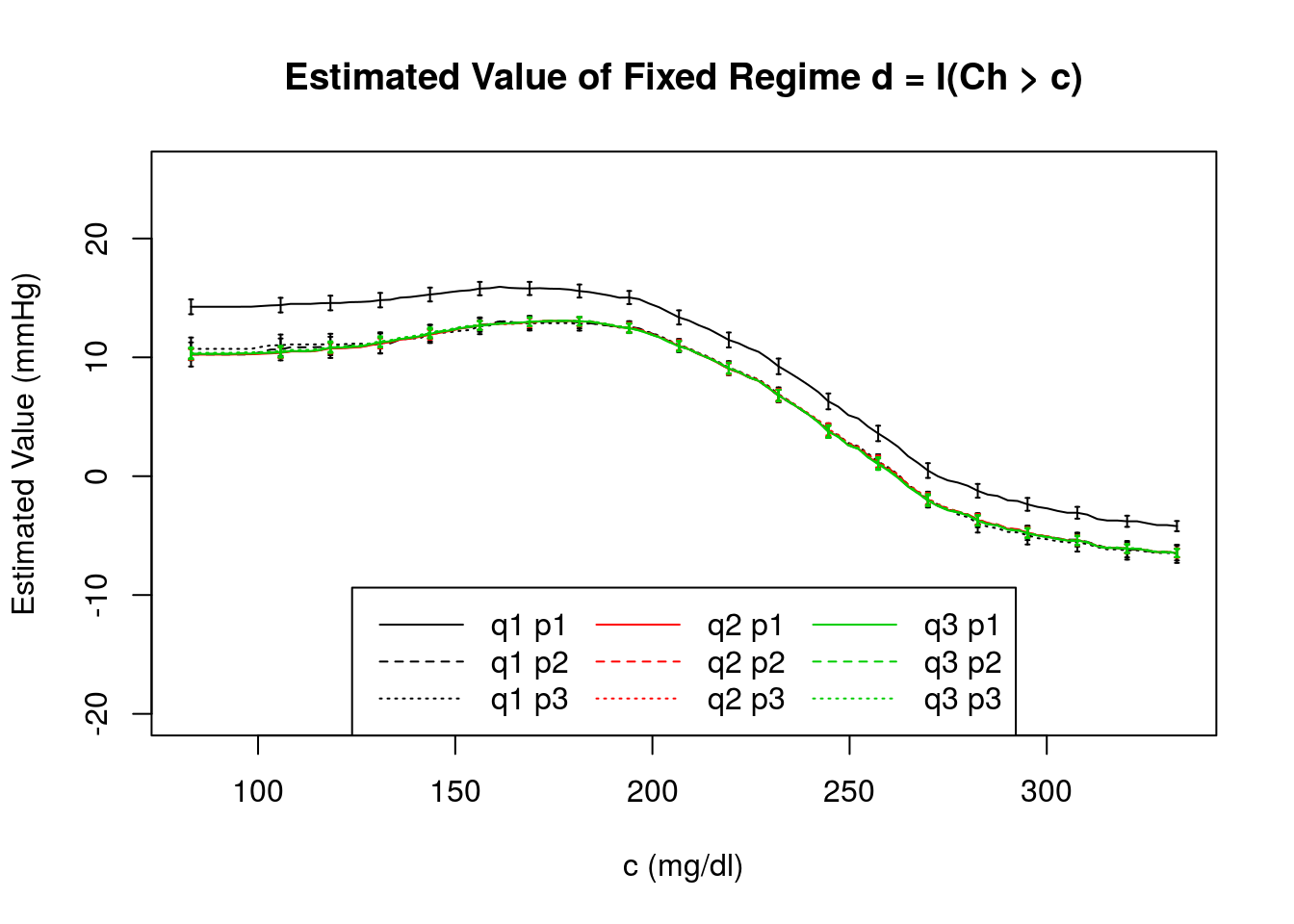
In this figure, we compare the estimated value of regime \(d = \{d_{1}(H_{1})\} = \text{I}(\text{Ch}>c)\}\) obtained using the AIPW estimator, \(\widehat{\mathcal{V}}_{AIPW}(d)\) and its standard error, \(\widehat{\sigma}_{11}\) obtained under each combination of the propensity score and outcome regression models under consideration. We see the estimates are very similar under each combination with the exception of the \(Q^{1}_{1}(h_{1},a_{1};\beta_{1})\) / \(\pi^{1}_{1}(h_{1};\gamma_{1})\) combination representing a case when both the propensity score and outcome regression models are completely misspecified. Again, we include the standard errors for only a subset of \(c\) for clarity of presentation.
Comparison of Estimators
The table below compares the estimated treatment effects and standard errors for all of the estimators discussed here and under all the models considered in this chapter.
| (mmHg) | \(\widehat{\mathcal{V}}_{IPW}(d)\) | \(Q^{1}_{1}(h_{1},a_{1};\beta_{1})\) | \(Q^{2}_{1}(h_{1},a_{1};\beta_{1})\) | \(Q^{3}_{1}(h_{1},a_{1};\beta_{1})\) |
| \(\widehat{\mathcal{V}}_{OR}(d)\) | — | 14.26 (0.62) | 10.21 (0.45) | 10.24 (0.45) |
| \(\pi^{1}_{1}(h_{1};\gamma_{1})\) | 14.23 (0.94) | 14.23 (0.62) | 10.19 (0.45) | 10.24 (0.45) |
| \(\pi^{2}_{1}(h_{1};\gamma_{1})\) | 10.21 (0.82) | 10.24 (1.01) | 10.22 (0.45) | 10.26 (0.45) |
| \(\pi^{3}_{1}(h_{1};\gamma_{1})\) | 10.45 (0.80) | 10.71 (0.95) | 10.26 (0.46) | 10.34 (0.45) |
The estimated standard errors are shown in parentheses. The first row contains \(\widehat{\mathcal{V}}_{OR}(d)\) estimated under each outcome regression model. The first column corresponds to \(\widehat{\mathcal{V}}_{IPW}(d)\) under each propensity score regression model. The shaded elements show \(\widehat{\mathcal{V}}_{AIPW}(d)\) for each combination of outcome and propensity score models.
We see that the estimated treatment effect tends to be smaller with less variance for methods that use the correctly specified outcome regression model, \(Q^{3}_{1}(h_{1},a_{1};\widehat{\beta}_{1})\).
The table below compares the estimated treatment effects and standard errors for all of the estimators discussed here and under all the models considered in this chapter.
| (mmHg) | \(\widehat{\mathcal{V}}_{IPW}(d)\) | \(Q^{1}_{1}(h_{1},a_{1};\beta_{1})\) | \(Q^{2}_{1}(h_{1},a_{1};\beta_{1})\) | \(Q^{3}_{1}(h_{1},a_{1};\beta_{1})\) |
| \(\widehat{\mathcal{V}}_{OR}(d)\) | — | -4.18 (0.43) | -6.43 (0.36) | -6.46 (0.34) |
| \(\pi^{1}_{1}(h_{1};\gamma_{1})\) | -4.20 (0.47) | -4.20 (0.43) | -6.46 (0.36) | -6.47 (0.34) |
| \(\pi^{2}_{1}(h_{1};\gamma_{1})\) | -6.45 (0.74) | -6.46 (0.62) | -6.48 (0.36) | -6.48 (0.34) |
| \(\pi^{3}_{1}(h_{1};\gamma_{1})\) | -6.56 (0.93) | -6.53 (0.77) | -6.45 (0.39) | -6.43 (0.35) |
The estimated standard errors are shown in parentheses. The first row contains \(\widehat{\mathcal{V}}_{OR}(d)\) estimated under each outcome regression model. The first column corresponds to \(\widehat{\mathcal{V}}_{IPW}(d)\) under each propensity score regression model. The shaded elements show \(\widehat{\mathcal{V}}_{AIPW}(d)\) for each combination of outcome and propensity score models.
We see that the estimated treatment effect tends to be smaller with less variance for methods that use the correctly specified outcome regression model, \(Q^{3}_{1}(h_{1},a_{1};\widehat{\beta}_{1})\).

| (mmHg) | \(\widehat{\mathcal{V}}_{IPW}(d)\) | \(Q^{1}_{1}(h_{1},a_{1};\beta_{1})\) | \(Q^{2}_{1}(h_{1},a_{1};\beta_{1})\) | \(Q^{3}_{1}(h_{1},a_{1};\beta_{1})\) |
| \(\widehat{\mathcal{V}}_{OR}(d)\) | — | 14.99 (0.61); [0.61] | 10.60 (0.47); [0.47] | 10.60 (0.46); [0.46] |
| \(\pi^{1}_{1}(h_{1};\gamma_{1})\) | 15.00 (0.61); [0.61] | 15.00 (0.61); [0.61] | 10.60 (0.47); [0.47] | 10.60 (0.46); [0.46] |
| \(\pi^{2}_{1}(h_{1};\gamma_{1})\) | 10.61 (0.53); [0.53] | 10.63 (0.58); [0.58] | 10.60 (0.47); [0.47] | 10.60 (0.46); [0.46] |
| \(\pi^{3}_{1}(h_{1};\gamma_{1})\) | 10.61 (0.63); [0.63] | 10.63 (0.79); [0.79] | 10.60 (0.48); [0.48] | 10.61 (0.47); [0.47] |
We see that the estimated values and standard errors are similar for the incomplete and true propensity score and/or outcome models.
| (mmHg) | \(\widehat{\mathcal{V}}_{IPW}(d)\) | \(Q^{1}_{1}(h_{1},a_{1};\beta_{1})\) | \(Q^{2}_{1}(h_{1},a_{1};\beta_{1})\) | \(Q^{3}_{1}(h_{1},a_{1};\beta_{1})\) |
| \(\widehat{\mathcal{V}}_{OR}(d)\) | — | -4.28 (0.44); [0.44] | -6.80 (0.38); [0.38] | -6.79 (0.35); [0.35] |
| \(\pi^{1}_{1}(h_{1};\gamma_{1})\) | -4.28 (0.44); [0.44] | -4.28 (0.44); [0.44] | -6.80 (0.38); [0.38] | -6.79 (0.35); [0.35] |
| \(\pi^{2}_{1}(h_{1};\gamma_{1})\) | -6.79 (0.43); [0.43] | -6.78 (0.42); [0.42] | -6.80 (0.38); [0.38] | -6.79 (0.35); [0.35] |
| \(\pi^{3}_{1}(h_{1};\gamma_{1})\) | -6.80 (0.58); [0.58] | -6.80 (0.54); [0.54] | -6.80 (0.41); [0.41] | -6.79 (0.36); [0.36] |
We see that the estimated values and standard errors are similar for the incomplete and true propensity score and/or outcome models.

\(Q_{1}(h_{1}, a_{1};\beta_{1})\)
Throughout Chapters 2-4, we consider three outcome regression models selected to represent a range of model (mis)specification. Note that we are not demonstrating a definitive analysis that one might do in practice, in which the analyst would use all sorts of variable selection techniques, etc., to arrive at a posited model. Rather, our objective is to illustrate how the methods work under a range of model (mis)specification.
Click on each tab below to see the model and basic model diagnostic steps. Note that this information was discussed previously in Chapter 2 and is repeated here for convenience.
The first model is a completely misspecified model
\[ Q^{1}_{1}(h_{1},a_{1};\beta_{1}) = \beta_{10} + \beta_{11} \text{W} + \beta_{12} \text{Cr} + a_{1}~(\beta_{13} + \beta_{14} \text{Cr}). \]
Modeling Object
The parameters of this model will be estimated using ordinary least squares via
The modeling objects for this regression step is
q1 <- modelObj::buildModelObj(model = ~ W + A*Cr,
solver.method = 'lm',
predict.method = 'predict.lm')Model Diagnostics
Though ultimately, the regression steps will be performed within the implementations of the treatment effect and value estimators, we make use of modelObj::
For \(Q^{1}_{1}(h_{1},a_{1};\beta_{1})\) the regression can be completed as follows
OR1 <- modelObj::fit(object = q1, data = dataSBP, response = y)
OR1 <- modelObj::fitObject(object = OR1)
OR1
Call:
lm(formula = YinternalY ~ W + A + Cr + A:Cr, data = data)
Coefficients:
(Intercept) W A Cr A:Cr
-6.66893 0.02784 16.46653 0.56324 2.41004 where for convenience we have made use of modelObj’s
Let’s examine the regression results for the model under consideration. First, the diagnostic plots defined for “lm” objects.
par(mfrow = c(2,2))
graphics::plot(x = OR1)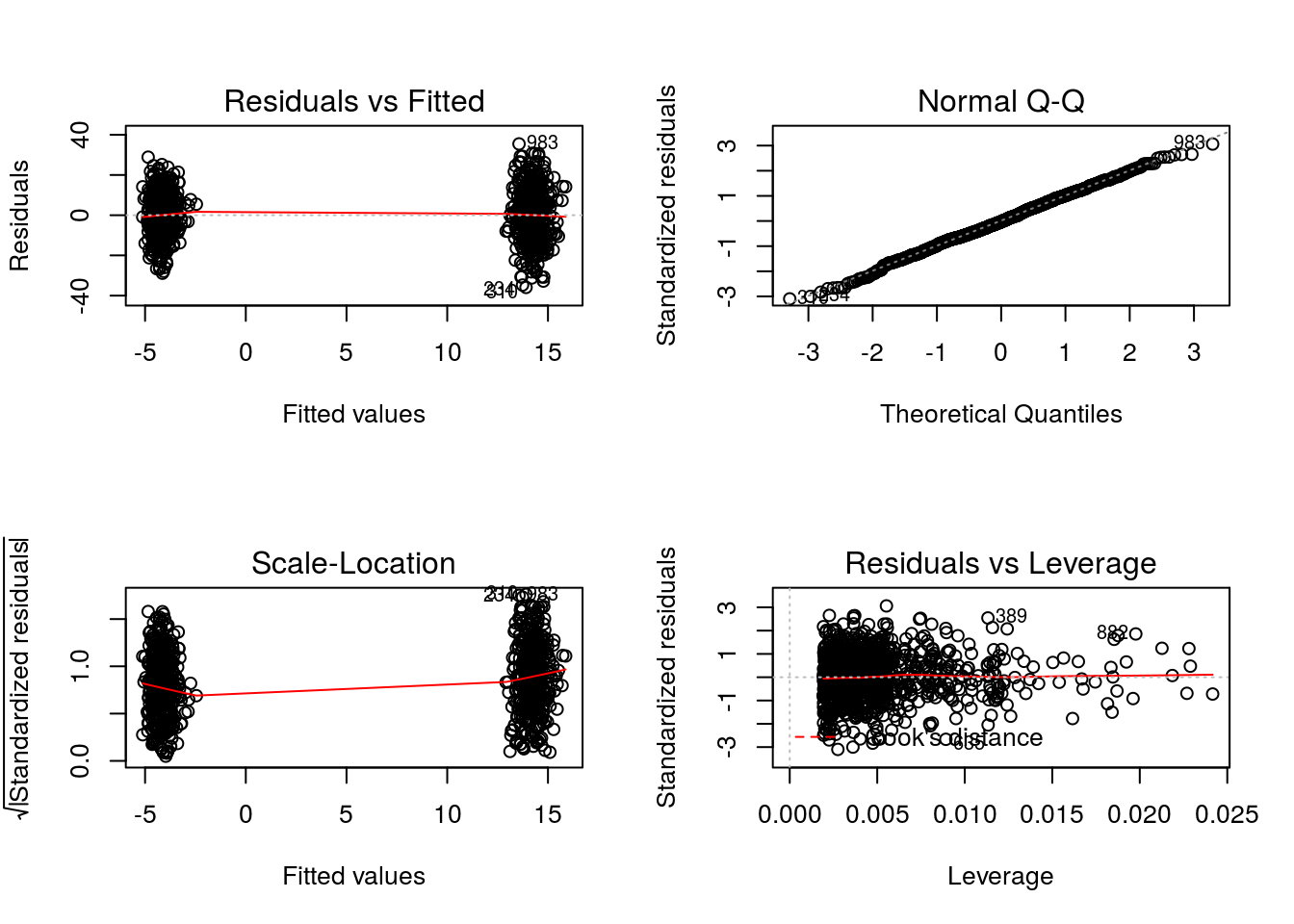
We see that the diagnostic plots for model \(Q^{1}_{1}(h_{1},a_{1};\beta_{1})\) show some unusual behaviors. The two groupings of residuals in the Residuals vs Fitted and the Scale-Location plots are reflecting the fact that the model includes only the covariates W and Cr, neither of which are associated with outcome in the true regression relationship. Thus, for all practical purposes the model is fitting the two treatment means.
Now, let’s examine the summary statistics for the regression step
summary(object = OR1)
Call:
lm(formula = YinternalY ~ W + A + Cr + A:Cr, data = data)
Residuals:
Min 1Q Median 3Q Max
-35.911 -7.605 -0.380 7.963 35.437
Coefficients:
Estimate Std. Error t value Pr(>|t|)
(Intercept) -6.66893 4.67330 -1.427 0.15389
W 0.02784 0.02717 1.025 0.30564
A 16.46653 5.96413 2.761 0.00587 **
Cr 0.56324 5.07604 0.111 0.91167
A:Cr 2.41004 7.22827 0.333 0.73889
---
Signif. codes: 0 '***' 0.001 '**' 0.01 '*' 0.05 '.' 0.1 ' ' 1
Residual standard error: 11.6 on 995 degrees of freedom
Multiple R-squared: 0.3853, Adjusted R-squared: 0.3828
F-statistic: 155.9 on 4 and 995 DF, p-value: < 2.2e-16We see that the residual standard error is large and that the adjusted R-squared value is small.
Readers familiar with R might have noticed that the response variable specified in the call to the regression method is
The second model is an incomplete model having only one of the covariates of the true model,
\[ Q^{2}_{1}(h_{1},a_{1};\beta_{1}) = \beta_{10} + \beta_{11} \text{Ch} + a_{1}~(\beta_{12} + \beta_{13} \text{Ch}). \]
Modeling Object
As for \(Q^{1}_{1}(h_{1},a_{1};\beta_{1})\), the parameters of this model will be estimated using ordinary least squares via
The modeling object for this regression step is
q2 <- modelObj::buildModelObj(model = ~ Ch*A,
solver.method = 'lm',
predict.method = 'predict.lm')Model Diagnostics
For \(Q^{2}_{1}(h_{1},a_{1};\beta_{1})\) the regression can be completed as follows
OR2 <- modelObj::fit(object = q2, data = dataSBP, response = y)
OR2 <- modelObj::fitObject(object = OR2)
OR2
Call:
lm(formula = YinternalY ~ Ch + A + Ch:A, data = data)
Coefficients:
(Intercept) Ch A Ch:A
36.5101 -0.2052 -89.5245 0.5074 where for convenience we have made use of modelObj’s
First, let’s examine the diagnostic plots defined for “lm” objects.
par(mfrow = c(2,4))
graphics::plot(x = OR2)
graphics::plot(x = OR1)
where we have included the diagnostic plots for model \(Q^{1}_{1}(h_{1},a_{1};\beta_{1})\) for easy comparison. We see that the residuals from the fit of model \(Q^{2}_{1}(h_{1},a_{1};\beta_{1})\) do not exhibit the two groupings, reflecting the fact that \(Q^{2}_{1}(h_{1},a_{1};\beta_{1})\) is only partially misspecified in that it includes the important covariate Ch.
Now, let’s examine the summary statistics for the regression step
summary(object = OR2)
Call:
lm(formula = YinternalY ~ Ch + A + Ch:A, data = data)
Residuals:
Min 1Q Median 3Q Max
-16.1012 -2.7476 -0.0032 2.6727 15.1825
Coefficients:
Estimate Std. Error t value Pr(>|t|)
(Intercept) 36.510110 0.933019 39.13 <2e-16 ***
Ch -0.205226 0.004606 -44.56 <2e-16 ***
A -89.524507 1.471905 -60.82 <2e-16 ***
Ch:A 0.507374 0.006818 74.42 <2e-16 ***
---
Signif. codes: 0 '***' 0.001 '**' 0.01 '*' 0.05 '.' 0.1 ' ' 1
Residual standard error: 4.511 on 996 degrees of freedom
Multiple R-squared: 0.907, Adjusted R-squared: 0.9068
F-statistic: 3239 on 3 and 996 DF, p-value: < 2.2e-16Comparing to the diagnostics for model \(Q^{1}_{1}(h_{1},a_{1};\beta_{1})\), we see that the residual standard error is smaller (4.51 vs 11.6) and that the adjusted R-squared value is larger (0.91 vs 0.38). Both of these results indicate that model \(Q^{2}_{1}(h_{1},a_{1};\beta_{1})\) is a more suitable model for \(E(Y|X=x,A=a)\) than model \(Q^{1}_{1}(h_{1},a_{1};\beta_{1})\).
The third model we will consider is the correctly specified model used to generate the dataset,
\[ Q^{3}_{1}(h_{1},a_{1};\beta_{1}) = \beta_{10} + \beta_{11} \text{Ch} + \beta_{12} \text{K} + a_{1}~(\beta_{13} + \beta_{14} \text{Ch} + \beta_{15} \text{K}). \]
Modeling Object
As for \(Q^{1}_{1}(h_{1},a_{1};\beta_{1})\) and \(Q^{2}_{1}(h_{1},a_{1};\beta_{1})\), the parameters of this model will be estimated using ordinary least squares via
The modeling object for this regression step is
q3 <- modelObj::buildModelObj(model = ~ (Ch + K)*A,
                              solver.method = 'lm',
predict.method = 'predict.lm')Model Diagnostics
For \(Q^{3}_{1}(h_{1},a_{1};\beta_{1})\) the regression can be completed as follows
OR3 <- modelObj::fit(object = q3, data = dataSBP, response = y)
OR3 <- modelObj::fitObject(object = OR3)
OR3
Call:
lm(formula = YinternalY ~ Ch + K + A + Ch:A + K:A, data = data)
Coefficients:
(Intercept) Ch K A Ch:A
-15.6048 -0.2035 12.2849 -61.0979 0.5048
K:A
-6.6099 where for convenience we have made use of modelObj’s
Again, let’s start by examining the diagnostic plots defined for “lm” objects.
par(mfrow = c(2,4))
graphics::plot(x = OR3)
graphics::plot(x = OR2)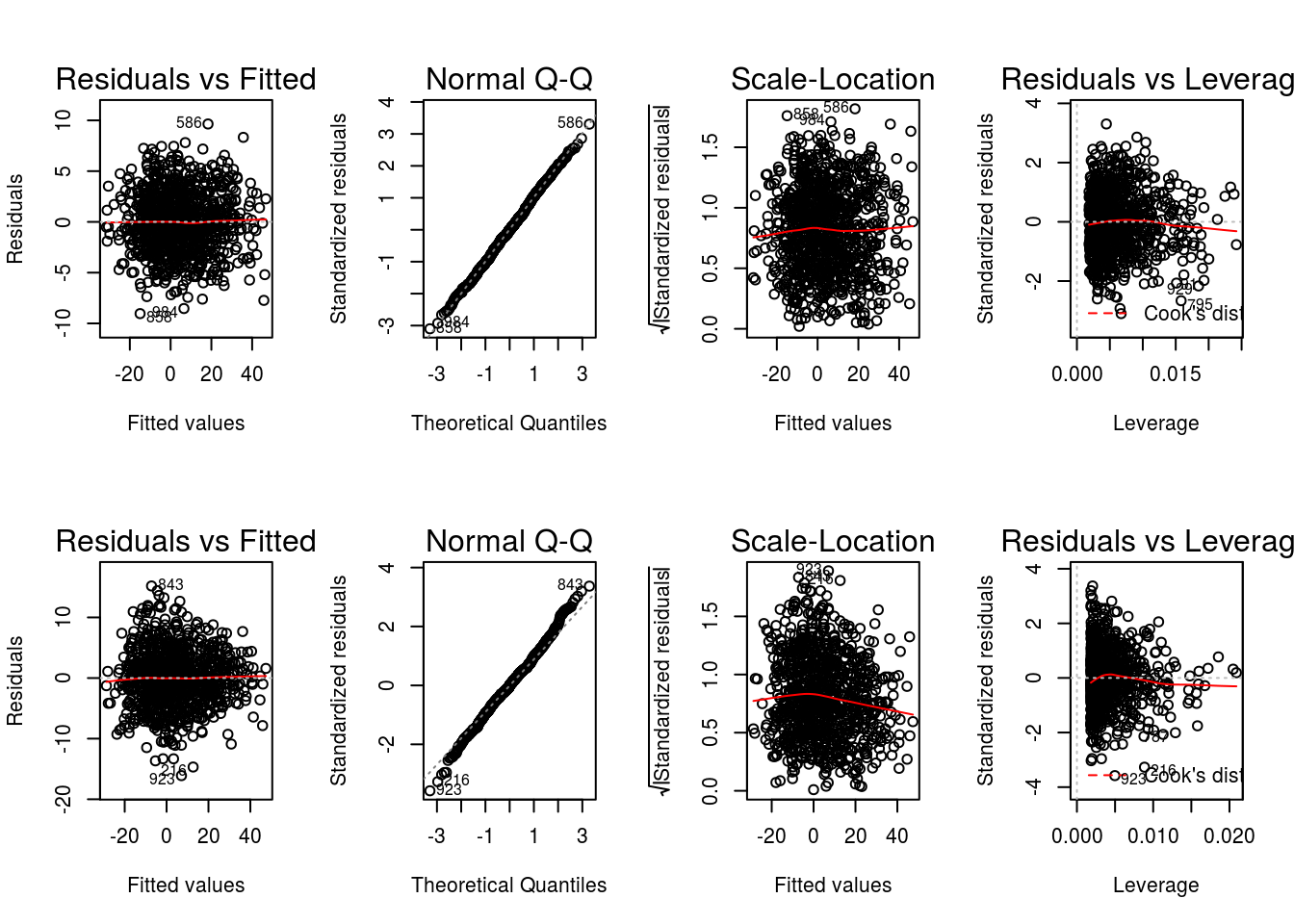
where we have included the diagnostic plots for model \(Q^{2}_{1}(h_{1},a_{1};\beta_{1})\) for easy comparison. We see that the results for models \(Q^{2}_{1}(h_{1},a_{1};\beta_{1})\) and \(Q^{3}_{1}(h_{1},a_{1};\beta_{1})\) are very similar, with model \(Q^{3}_{1}(h_{1},a_{1};\beta_{1})\) yielding slightly better diagnostics (e.g., smaller residuals); a result in line with the knowledge that \(Q^{3}_{1}(h_{1},a_{1};\beta_{1})\) is the model used to generate the data.
Now, let’s examine the summary statistics for the regression step
summary(object = OR3)
Call:
lm(formula = YinternalY ~ Ch + K + A + Ch:A + K:A, data = data)
Residuals:
Min 1Q Median 3Q Max
-9.0371 -1.9376 0.0051 2.0127 9.6452
Coefficients:
Estimate Std. Error t value Pr(>|t|)
(Intercept) -15.604845 1.636349 -9.536 <2e-16 ***
Ch -0.203472 0.002987 -68.116 <2e-16 ***
K 12.284852 0.358393 34.278 <2e-16 ***
A -61.097909 2.456637 -24.871 <2e-16 ***
Ch:A 0.504816 0.004422 114.168 <2e-16 ***
K:A -6.609876 0.538386 -12.277 <2e-16 ***
---
Signif. codes: 0 '***' 0.001 '**' 0.01 '*' 0.05 '.' 0.1 ' ' 1
Residual standard error: 2.925 on 994 degrees of freedom
Multiple R-squared: 0.961, Adjusted R-squared: 0.9608
F-statistic: 4897 on 5 and 994 DF, p-value: < 2.2e-16As for model \(Q^{2}_{1}(h_{1},a_{1};\beta_{1})\), we see that the residual standard error is smaller (2.93 vs 4.51) and that the adjusted R-squared value is larger (0.96 vs 0.91). Again, these results indicate that model \(Q^{3}_{1}(h_{1},a_{1};\beta_{1})\) is a more suitable model than both models \(Q^{1}_{1}(h_{1},a_{1};\beta_{1})\) and \(Q^{2}_{1}(h_{1},a_{1};\beta_{1})\).
\(\pi_{1}(h_{1};\gamma_{1})\)
Throughout Chapters 2-4, we consider three propensity score models selected to represent a range of model (mis)specification. Note that we are not demonstrating a definitive analysis that one might do in practice, in which the analyst would use all sorts of variable selection techniques, etc., to arrive at a posited model. Our objective is to illustrate how the methods work under a range of model (mis)specification.
Click on each tab below to see the model and basic model diagnostic steps. Note that this information was discussed previously in Chapter 2 and is repeated here for convenience.
The first model is a completely misspecified model having none of the covariates used in the data generating model
\[ \pi^{1}_{1}(h_{1};\gamma_{1}) = \frac{\exp(\gamma_{10} + \gamma_{11}~\text{W} + \gamma_{12}~\text{Cr})}{1+\exp(\gamma_{10} + \gamma_{11}~\text{W} + \gamma_{12}~\text{Cr})}. \]
Modeling Object
The parameters of this model will be estimated using maximum likelihood via
p1 <- modelObj::buildModelObj(model = ~ W + Cr,
solver.method = 'glm',
solver.args = list(family='binomial'),
predict.method = 'predict.glm',
predict.args = list(type='response'))Model Diagnostics
Though we will implement our treatment effect and value estimators in such a way that the regression step is performed internally, it is convenient to do model diagnostics separately here. We will make use of modelObj::
For \(\pi^{1}_{1}(h_{1};\gamma_{1})\) the regression can be completed as follows:
PS1 <- modelObj::fit(object = p1, data = dataSBP, response = dataSBP$A)
PS1 <- modelObj::fitObject(object = PS1)
PS1
Call: glm(formula = YinternalY ~ W + Cr, family = "binomial", data = data)
Coefficients:
(Intercept) W Cr
0.966434 -0.007919 -0.703766
Degrees of Freedom: 999 Total (i.e. Null); 997 Residual
Null Deviance: 1378
Residual Deviance: 1374 AIC: 1380where for convenience we have made use of modelObj’s
Now, let’s examine the regression results for the model under consideration.
summary(object = PS1)
Call:
glm(formula = YinternalY ~ W + Cr, family = "binomial", data = data)
Deviance Residuals:
Min 1Q Median 3Q Max
-1.239 -1.104 -1.027 1.248 1.443
Coefficients:
Estimate Std. Error z value Pr(>|z|)
(Intercept) 0.966434 0.624135 1.548 0.1215
W -0.007919 0.004731 -1.674 0.0942 .
Cr -0.703766 0.627430 -1.122 0.2620
---
Signif. codes: 0 '***' 0.001 '**' 0.01 '*' 0.05 '.' 0.1 ' ' 1
(Dispersion parameter for binomial family taken to be 1)
Null deviance: 1377.8 on 999 degrees of freedom
Residual deviance: 1373.8 on 997 degrees of freedom
AIC: 1379.8
Number of Fisher Scoring iterations: 4First, in comparing the null deviance (1377.8) and the residual deviance (1373.8), we see that including the independent variables does not significantly reduce the deviance. Thus, this model is not significantly better than the constant propensity score model. However, we know that the data mimics an observational study for which the propensity score is not constant or known. And, note that the Akaike Information Criterion (AIC) is large (1379.772). Though the AIC value alone does not tell us much about the quality of our model, we can compare this to other models to determine a relative quality.
The second model is an incomplete model having only one of the covariates of the true data generating model
\[ \pi^{2}_{1}(h_{1};\gamma_{1}) = \frac{\exp(\gamma_{10} + \gamma_{11} \text{Ch})}{1+\exp(\gamma_{10} + \gamma_{11} \text{Ch})}. \]
Modeling Object
As for \(\pi_{1}(h_{1};\gamma)\) the parameters of this model will be estimated using maximum likelihood via
The modeling objects for this regression step is
p2 <- modelObj::buildModelObj(model = ~ Ch,
solver.method = 'glm',
solver.args = list(family='binomial'),
predict.method = 'predict.glm',
predict.args = list(type='response'))The regression is completed as follows:
PS2 <- modelObj::fit(object = p2, data = dataSBP, response = dataSBP$A)
PS2 <- modelObj::fitObject(object = PS2)
PS2
Call: glm(formula = YinternalY ~ Ch, family = "binomial", data = data)
Coefficients:
(Intercept) Ch
-3.06279 0.01368
Degrees of Freedom: 999 Total (i.e. Null); 998 Residual
Null Deviance: 1378
Residual Deviance: 1298 AIC: 1302Again, we use
summary(PS2)
Call:
glm(formula = YinternalY ~ Ch, family = "binomial", data = data)
Deviance Residuals:
Min 1Q Median 3Q Max
-1.7497 -1.0573 -0.7433 1.1449 1.9316
Coefficients:
Estimate Std. Error z value Pr(>|z|)
(Intercept) -3.062786 0.348085 -8.799 <2e-16 ***
Ch 0.013683 0.001617 8.462 <2e-16 ***
---
Signif. codes: 0 '***' 0.001 '**' 0.01 '*' 0.05 '.' 0.1 ' ' 1
(Dispersion parameter for binomial family taken to be 1)
Null deviance: 1377.8 on 999 degrees of freedom
Residual deviance: 1298.2 on 998 degrees of freedom
AIC: 1302.2
Number of Fisher Scoring iterations: 4First, in comparing the null deviance (1377.8) and the residual deviance (1298.2), we see that including the independent variables leads to a smaller deviance than obtained from the intercept only model. And finally, we see that the AIC is large (1302.247), but it is less than that obtained for \(\pi^{1}_{1}(h_{1};\gamma_{1})\) (1379.772). This result is not unexpected as we know that the model is only partially misspecified.
The third model we will consider is the correctly specified model used to generate the data set,
\[ \pi^{3}_{1}(h_{1};\gamma_{1}) = \frac{\exp(\gamma_{10} + \gamma_{11}~\text{SBP0} + \gamma_{12}~\text{Ch})}{1+\exp(\gamma_{10} + \gamma_{11}~\text{SBP0}+ \gamma_{12}~\text{Ch})}. \]
The parameters of this model will be estimated using maximum likelihood via
The modeling objects for this regression step is
p3 <- modelObj::buildModelObj(model = ~ SBP0 + Ch,
                              solver.method = 'glm',
                              solver.args = list(family='binomial'),
                              predict.method = 'predict.glm',
predict.args = list(type='response'))The regression is completed as follows:
PS3 <- modelObj::fit(object = p3, data = dataSBP, response = dataSBP$A)
PS3 <- modelObj::fitObject(object = PS3)
PS3
Call:  glm(formula = YinternalY ~ SBP0 + Ch, family = "binomial", data = data)

Coefficients:
(Intercept)         SBP0           Ch
  -15.94153      0.07669      0.01589

Degrees of Freedom: 999 Total (i.e. Null);  997 Residual
Null Deviance:      1378
Residual Deviance: 1162     AIC: 1168
Again, we use
summary(PS3)
Call:
glm(formula = YinternalY ~ SBP0 + Ch, family = "binomial", data = data)

Deviance Residuals:
    Min       1Q   Median       3Q      Max
-2.3891  -0.9502  -0.4940   0.9939   2.1427

Coefficients:
              Estimate Std. Error z value Pr(>|z|)
(Intercept) -15.941527   1.299952 -12.263   <2e-16 ***
SBP0          0.076687   0.007196  10.657   <2e-16 ***
Ch            0.015892   0.001753   9.066   <2e-16 ***
---
Signif. codes:  0 '***' 0.001 '**' 0.01 '*' 0.05 '.' 0.1 ' ' 1

(Dispersion parameter for binomial family taken to be 1)

    Null deviance: 1377.8  on 999  degrees of freedom
Residual deviance: 1161.6  on 997  degrees of freedom
AIC: 1167.6

Number of Fisher Scoring iterations: 3
First, we see from the null deviance (1377.8) and the residual deviance (1161.6) that including the independent variables does reduce the deviance as compared to the intercept only model. And finally, we see that the AIC is large (1167.621), but it is less than that obtained for both \(\pi^{1}_{1}(h_{1};\gamma_{1})\) (1379.772) and \(\pi^{2}_{1}(h_{1};\gamma_{1})\) (1302.247). This result is in-line with the knowledge that this is the data generating model.