
Regression Based Estimator
The regression-based approach to estimate the value of \(\Psi\)-specific fixed regime \(d = (d_{1}(h_{1}), d_{2}(h_{2}), \dots, d_{K}(h_{K}))\), \(\widehat{\mathcal{V}}_{Q}(d)\), is as follows.
Start at Decision \(K\). For \((h_{K}, a_{K}) = (\overline{x}_{k}, \overline{a}_{K})\) define
\[ Q_{K}^{d}(h_{K},a_{K}) = E(Y|H_{K} = h_{K}, A_{K} = a_{K}), \] and let
\[ V_{K}^{d}(h_{K}) = Q_{K}^{d}\left\{h_{K}, d_{K}(h_{K})\right\}, \] which is \(Q_{K}^{d}(h_{K},a_{K})\) evaluated at \(a_{K} = d_{K}(h_{K})\).
We posit a model for \(Q_{K}^{d}(h_{K},a_{K})\), \(Q_{K}^{d}(h_{K},a_{K};\beta_{K})\) and solve a suitable M-estimating equation to estimate \(\beta_{K}\), \(\widehat{\beta}_{K}\). Once we have a fitted model, \(Q_{K}^{d}(h_{K},a_{K}; \widehat{\beta}_{K})\), form pseudo outcomes
\[ \widetilde{V}_{Ki}^{d} = Q_{K}^{d}\left\{H_{Ki}, d_{K}(H_{Ki}); \widehat{\beta}_{K}\right\}, \quad i = 1, \dots, n, \] which are the predicted outcomes based on the fitted model if each individual were to have received treatment according to rule \(d_{K}\) at Decision \(K\).
Now consider Decision \(K-1\). Posit a parametric model for \(Q_{K-1}^{d}(h_{K-1},a_{K-1})\), \(Q_{K-1}^{d}(h_{K-1},a_{K-1};\beta_{K-1})\) for
\[ E\left\{V_{K}^{d}(H_{K})|H_{K-1} = h_{K-1}, A_{K-1} = a_{K-1}\right\}, \]
and solve a suitable M-estimating equation to obtain the estimator \(\widehat{\beta}_{K-1}\) for \(\beta_{K-1}\). Once we have a fitted model, \(Q_{K-1}^{d}(h_{K-1},a_{K-1}; \widehat{\beta}_{K-1})\), form pseudo outcomes
\[ \widetilde{V}_{K-1,i}^{d} = Q_{K-1}^{d}\left\{H_{K-1,i}, d_{K-1}(H_{K-1,i}); \widehat{\beta}_{K-1}\right\}, \quad i = 1, \dots, n. \]
Continue in this fashion for each \(k=K-2,\dots,1\). Finally, the estimator for the value \(\mathcal{V}(d)\) is
\[ \widehat{\mathcal{V}}(d) = n^{-1} \sum_{i=1}^{n} \widetilde{V}_{1i}^{d}. \]
This approach is the “backward induction” approach discussed in the book. An alternative approach is that of “monotone coarsening,” which we do not discuss here.
We define function
#------------------------------------------------------------------------------#
# regression based estimator for value of a fixed tx regime with feasible tx
#   sets at each of the K>1 decision points
#
# ASSUMPTIONS
#   each tx is coded as {0,1}
#
# INPUTS
#  moQ    : list of modeling objects for Q-function regressions
#           kth element corresponds to kth decision point
#  data   : data.frame containing all covariates and txs
#  y      : outcome of interest
#  txName : vector of tx names (each tx must be coded as 0/1)
#  regime : matrix of 0/1 containing recommended txs
#           kth column corresponds to kth decision point
#
# RETURNS
#  a list containing
#      fitQ : list of value objects returned by Q-function regressions
#  valueHat : estimated value
#------------------------------------------------------------------------------#
value_Q_md <- function(moQ, data, y, txName, regime) {

  # number of decision points
  K <- length(x = moQ)

  #### Q-function Regressions

  qStep <- function(moQ, data, y, txName, regime) {
    # fit Q-function model
    fitObj <- modelObj::fit(object = moQ, data = data, response = y)

    # set tx received to recommended tx
    data[,txName] <- regime

    # predict Q-function for recommended tx
    qk <- modelObj::predict(object = fitObj, newdata = data)

    return (list("fit" = fitObj, "qk" = qk))
  }

  fitQ <- list()
  response <- y

  for (k in K:2L) {

    ### consider only individual with more than 1 tx option
    one <- data[,txName[k-1L]] == 1L

    ## kth Q-function regression

    sk <- qStep(moQ = moQ[[ k ]],
                data = data[!one,,drop = FALSE],
                y = response[!one],
                txName = txName[k],
                regime = regime[!one,k])

    fitQ[[ k ]] <- sk$fit
    response[!one] <- sk$qk

  }

  ## k=1 Q-function regression

  s1 <- qStep(moQ = moQ[[ 1L ]],
              data = data,
              y = response,
              txName = txName[1L],
              regime = regime[,1L])

  fitQ[[ 1L ]] <- s1$fit
  response <- s1$qk

  value <- mean(x = response)

  return( list("fitQ" = fitQ, "valueHat" = value) )
}
With
As was done in Chapter 5, we compare the estimated value under a variety of fixed regimes. Each tab below illustrates how to define the fixed regime under consideration and complete an analysis using the posited Q-function models.
The first fixed regime we consider is the static regime \(d = \{d_{1}(x_{1}) \equiv 1, d_{2}(\overline{x}_{2}) \equiv 1, d_{3}(\overline{x}_{3}) \equiv 1\}\). That is, all individuals are recommended to receive treatment \(A_{k} = 1\), \(k = 1, 2, 3\).
The estimated value of this fixed regime is obtained as follows:
q1 <- modelObj::buildModelObj(model = ~ CD4_0*A1,
                              solver.method = 'lm',
                              predict.method = 'predict.lm')
q2 <- modelObj::buildModelObj(model = ~ CD4_0 + CD4_6*A2,
solver.method = 'lm',
predict.method = 'predict.lm')q3 <- modelObj::buildModelObj(model = ~ CD4_0 + CD4_6 + CD4_12*A3,
solver.method = 'lm',
predict.method = 'predict.lm')regime <- matrix(data = 1L, nrow = nrow(x = dataMDPF), ncol = 3L)value_Q_md(moQ = list(q1, q2, q3),
data = dataMDPF,
y = dataMDPF$Y,
txName = c("A1","A2","A3"),
regime = regime)$fitQ
$fitQ[[1]]
Call:
lm(formula = YinternalY ~ CD4_0 + A1 + CD4_0:A1, data = data)
Coefficients:
(Intercept) CD4_0 A1 CD4_0:A1
846.727405 -0.305528 10.459837 0.006195
$fitQ[[2]]
Call:
lm(formula = YinternalY ~ CD4_0 + CD4_6 + A2 + CD4_6:A2, data = data)
Coefficients:
(Intercept) CD4_0 CD4_6 A2 CD4_6:A2
923.4224 2.0372 -1.8156 -78.5422 -0.0542
$fitQ[[3]]
Call:
lm(formula = YinternalY ~ CD4_0 + CD4_6 + CD4_12 + A3 + CD4_12:A3,
data = data)
Coefficients:
(Intercept) CD4_0 CD4_6 CD4_12 A3 CD4_12:A3
317.3743 2.0326 0.1371 -0.4478 603.5614 -1.9814
$valueHat
[1] 723.2833We see that the regression based estimator of the value under \(d = \{d_{1}(x_{1}) \equiv 1, d_{2}(\overline{x}_{2}) \equiv 1, d_{3}(\overline{x}_{3}) \equiv 1\}\) is 723.28 cells/mm\(^3\).
The second fixed regime we consider is the static regime \(d = \{d_{1}(x_{1}) \equiv 0, d_{2}(\overline{x}_{2}) \equiv 0, d_{3}(\overline{x}_{3}) \equiv 0\}\). That is, all individuals are recommended to receive treatment \(A_{k} = 0\), \(k = 1, 2, 3\).
The estimated value of this fixed regime and its standard error are obtained as follows:
q1 <- modelObj::buildModelObj(model = ~ CD4_0*A1,
solver.method = 'lm',
predict.method = 'predict.lm')q2 <- modelObj::buildModelObj(model = ~ CD4_0 + CD4_6*A2,
solver.method = 'lm',
predict.method = 'predict.lm')q3 <- modelObj::buildModelObj(model = ~ CD4_0 + CD4_6 + CD4_12*A3,
solver.method = 'lm',
predict.method = 'predict.lm')regime <- matrix(data = 0L, nrow = nrow(x = dataMDPF), ncol = 3L)value_Q_md(moQ = list(q1, q2, q3),
data = dataMDPF,
y = dataMDPF$Y,
txName = c("A1","A2","A3"),
regime = regime)$fitQ
$fitQ[[1]]
Call:
lm(formula = YinternalY ~ CD4_0 + A1 + CD4_0:A1, data = data)
Coefficients:
(Intercept) CD4_0 A1 CD4_0:A1
318.206 1.754 538.981 -2.053
$fitQ[[2]]
Call:
lm(formula = YinternalY ~ CD4_0 + CD4_6 + A2 + CD4_6:A2, data = data)
Coefficients:
(Intercept) CD4_0 CD4_6 A2 CD4_6:A2
318.0672 1.9303 -0.1408 527.2873 -1.6443
$fitQ[[3]]
Call:
lm(formula = YinternalY ~ CD4_0 + CD4_6 + CD4_12 + A3 + CD4_12:A3,
data = data)
Coefficients:
(Intercept) CD4_0 CD4_6 CD4_12 A3 CD4_12:A3
317.3743 2.0326 0.1371 -0.4478 603.5614 -1.9814
$valueHat
[1] 1102.807We see that the regression based estimator of the value under \(d = \{d_{1}(x_{1}) \equiv 0, d_{2}(\overline{x}_{2}) \equiv 0, d_{3}(\overline{x}_{3}) \equiv 0\}\) is 1102.81 cells/mm\(^3\).
The final fixed regime we consider is a covariate dependent regime
\[ d = \left\{ \begin{array}{l} d_{1}(x_{1}) = \text{I}(\text{CD4_0} < 250 ~\text{cells}/\text{mm}^{3}) \\ d_{2}(\overline{x}_{2}) = d_{1}(x_{1}) + \{1-d_{1}(x_{1})\} ~ \text{I}(\text{CD4_6} < 360 ~\text{cells}/\text{mm}^{3}) \\ d_{3}(\overline{x}_{2}) = d_{2}(\overline{x}_{2}) + \{1-d_{2}(\overline{x}_{2})\} ~ \text{I}(\text{CD4_12} < 300 ~\text{cells}/\text{mm}^{3}) \end{array} ~~~. \right. \]
The estimated value of this fixed regime and its standard error are obtained as follows:
q1 <- modelObj::buildModelObj(model = ~ CD4_0*A1,
solver.method = 'lm',
predict.method = 'predict.lm')q2 <- modelObj::buildModelObj(model = ~ CD4_0 + CD4_6*A2,
solver.method = 'lm',
predict.method = 'predict.lm')q3 <- modelObj::buildModelObj(model = ~ CD4_0 + CD4_6 + CD4_12*A3,
solver.method = 'lm',
predict.method = 'predict.lm')d1 <- as.integer(x = {dataMDPF$CD4_0 < 250.0})
d2 <- d1 + {1L-d1}*as.integer(x = {dataMDPF$CD4_6 < 360.0})
d3 <- d2 + {1L-d2}*as.integer(x = {dataMDPF$CD4_12 < 300.0})
regime <- cbind(d1, d2, d3)value_Q_md(moQ = list(q1, q2, q3),
data = dataMDPF,
y = dataMDPF$Y,
txName = c("A1","A2","A3"),
regime = regime)$fitQ
$fitQ[[1]]
Call:
lm(formula = YinternalY ~ CD4_0 + A1 + CD4_0:A1, data = data)
Coefficients:
(Intercept) CD4_0 A1 CD4_0:A1
372.657 1.646 484.531 -1.945
$fitQ[[2]]
Call:
lm(formula = YinternalY ~ CD4_0 + CD4_6 + A2 + CD4_6:A2, data = data)
Coefficients:
(Intercept) CD4_0 CD4_6 A2 CD4_6:A2
344.8571 1.8542 -0.1218 500.8351 -1.6030
$fitQ[[3]]
Call:
lm(formula = YinternalY ~ CD4_0 + CD4_6 + CD4_12 + A3 + CD4_12:A3,
data = data)
Coefficients:
(Intercept) CD4_0 CD4_6 CD4_12 A3 CD4_12:A3
317.3743 2.0326 0.1371 -0.4478 603.5614 -1.9814
$valueHat
[1] 1111.321We see that the regression based estimator of the value under this regime is 1111.32 cells/mm\(^3\).
Inverse Propensity Weighted Estimator
\[ \widehat{\mathcal{V}}_{IPW}(d) = n^{-1} \sum_{i=1}^{n} \frac{\mathcal{C}_{d,i}Y_{i}}{\left\{\prod_{k=2}^{K}\pi_{d,k}(\overline{X}_{ki});\widehat{\gamma}_{k})\right\}\pi_{d,1}(X_{1i};\widehat{\gamma}_{1})}. \] where
\[ \mathcal{C}_{d,i} = \text{I}\{\overline{A}_{i} = \overline{d}(\overline{X}_{i})\} \]
is the indicator of whether or not all treatments actually received coicides with the options dictated by \(d\). For binary treatments \(\mathcal{A}_{k} = \{0,1\}\), \(k=1, \dots, K\)
\[ \pi_{d,k}(h_{k}; \gamma_{k}) = \sum_{l=1}^{\ell_{k}}\text{I}\{s_{k}(h_{k}) = l\} \prod_{a_{k} = 1}^{m_{kl}} \omega_{k,l}(h_{k},a_{k};\gamma_{k})\text{I}\{d_{k}(h_{k}) = a_{k}\} \]
Recall that \(\omega_{k}(h_{k},a_{k}; \gamma_{k})\) is a model for
\[ \omega_{k}(h_{k},a_{k}) = P(A_{k} = a_{k} | H_{k} = h_{k}), \quad k = 1, \ldots, K. \]
We define function
#------------------------------------------------------------------------------#
# IPW estimator for value of a fixed tx regime with binary tx at each of the
# K>1 decision points
#
# ASSUMPTIONS
# each tx is binary coded as {0,1}
#
# INPUTS
# moPS : list of modeling objects for propensity score regressions
# kth element corresponds to kth decision point
# data : data.frame containing all covariates and txs
# *** each tx must be coded 0/1 ***
# y : outcome of interest
# txName : vector of tx names (each tx must be coded as 0/1)
# regime : matrix of 0/1 containing recommended txs
# kth column corresponds to kth decision point
#
# RETURNS
# a list containing
# fitPS : list of value objects returned by propensity score regression
# valueHat : estimated value
#------------------------------------------------------------------------------#
value_IPW_md <- function(moPS, data, y, txName, regime) {
# number of decision points
K <- length(x = moPS)
# number of patients in data set
n <- nrow(x = data)
#### Propensity Score Regressions
piStep <- function(moPS, data, y, regime) {
# fit propensity score model
fitObj <- modelObj::fit(object = moPS, data = data, response = y)
# predict propensity score
pk <- modelObj::predict(object = fitObj, newdata = data)
if (is.matrix(x = pk)) pk <- pk[,ncol(x = pk),drop = TRUE]
# pull propensity score corresponding to recommended treatment
pidk <- pk*{regime == 1L} + {1.0 - pk}*{regime == 0L}
return (list("fit" = fitObj, "pidk" = pidk))
}
fitPS <- list()
pid <- matrix(data = 1.0, nrow = n, ncol = K)
for (k in K:2L) {
# use only individuals with more than 1 tx option
one <- data[,txName[k-1L]] == 1L
## kth propensity score regression
sk <- piStep(moPS = moPS[[ k ]],
data = data[!one,,drop = FALSE],
y = data[!one,txName[k]],
regime = regime[!one,k])
fitPS[[ k ]] <- sk$fit
pid[!one,k] <- sk$pidk
}
## k=1 propensity score regression
s1 <- piStep(moPS = moPS[[ 1L ]],
data = data,
y = data[,txName[1L]],
regime = regime[,1L])
fitPS[[ 1L ]] <- s1$fit
pid[,1L] <- s1$pidk
# indicator of all txs received being those recommended
cee <- apply(X = {data[,txName] == regime}, MARGIN = 1L, FUN = prod)
# P(C == 1|H)
pid <- apply(X = pid, MARGIN = 1L, FUN = prod)
#### Value Estimate
value <- mean(x = cee * y / pid)
return( list("fitPS" = fitPS, "valueHat" = value) )
}With
We compare the estimated value under the fixed regimes considered for the regression based estimator. Each tab below illustrates how to define the fixed regime under consideration and complete an analysis using the posited propensity score models.
The first fixed regime we consider is the static regime \(d = \{d_{1}(x_{1}) \equiv 1, d_{2}(\overline{x}_{2}) \equiv 1, d_{3}(\overline{x}_{3}) \equiv 1\}\). That is, all individuals are recommended to receive treatment \(A_{k} = 1\), \(k = 1, 2, 3\).
The estimated value of this fixed regime and its standard error are obtained as follows:
p1 <- modelObj::buildModelObj(model = ~ CD4_0,
solver.method = 'glm',
solver.args = list(family='binomial'),
predict.method = 'predict.glm',
predict.args = list(type='response'))p2 <- modelObj::buildModelObj(model = ~ CD4_6,
solver.method = 'glm',
solver.args = list(family='binomial'),
predict.method = 'predict.glm',
predict.args = list(type='response'))p3 <- modelObj::buildModelObj(model = ~ CD4_12,
solver.method = 'glm',
solver.args = list(family='binomial'),
predict.method = 'predict.glm',
predict.args = list(type='response'))regime <- matrix(data = 1L, nrow = nrow(x = dataMDPF), ncol = 3L)value_IPW_md(moPS = list(p1, p2, p3),
data = dataMDPF,
y = dataMDPF$Y,
txName = c("A1","A2","A3"),
regime = regime)$fitPS
$fitPS[[1]]
Call: glm(formula = YinternalY ~ CD4_0, family = "binomial", data = data)
Coefficients:
(Intercept) CD4_0
2.385956 -0.006661
Degrees of Freedom: 999 Total (i.e. Null); 998 Residual
Null Deviance: 1316
Residual Deviance: 1227 AIC: 1231
$fitPS[[2]]
Call: glm(formula = YinternalY ~ CD4_6, family = "binomial", data = data)
Coefficients:
(Intercept) CD4_6
1.234491 -0.004781
Degrees of Freedom: 631 Total (i.e. Null); 630 Residual
Null Deviance: 608.5
Residual Deviance: 577.8 AIC: 581.8
$fitPS[[3]]
Call: glm(formula = YinternalY ~ CD4_12, family = "binomial", data = data)
Coefficients:
(Intercept) CD4_12
0.929409 -0.003816
Degrees of Freedom: 513 Total (i.e. Null); 512 Residual
Null Deviance: 622.5
Residual Deviance: 609.1 AIC: 613.1
$valueHat
[1] 716.5866We see that the inverse probability weighted estimator of the value under this regime is 716.59 cells/mm\(^3\). Note that 368 individuals in our data set followed this regime and thus contribute to the estimator.
The second fixed regime we consider is the static regime \(d = \{d_{1}(x_{1}) \equiv 0, d_{2}(\overline{x}_{2}) \equiv 0, d_{3}(\overline{x}_{3}) \equiv 0\}\). That is, all individuals are recommended to receive treatment \(A_{k} = 0\), \(k = 1, 2, 3\).
The estimated value of this fixed regime and its standard error are obtained as follows:
p1 <- modelObj::buildModelObj(model = ~ CD4_0,
solver.method = 'glm',
solver.args = list(family='binomial'),
predict.method = 'predict.glm',
predict.args = list(type='response'))p2 <- modelObj::buildModelObj(model = ~ CD4_6,
solver.method = 'glm',
solver.args = list(family='binomial'),
predict.method = 'predict.glm',
predict.args = list(type='response'))p3 <- modelObj::buildModelObj(model = ~ CD4_12,
solver.method = 'glm',
solver.args = list(family='binomial'),
predict.method = 'predict.glm',
predict.args = list(type='response'))regime <- matrix(data = 0L, nrow = nrow(x = dataMDPF), ncol = 3L)value_IPW_md(moPS = list(p1, p2, p3),
data = dataMDPF,
y = dataMDPF$Y,
txName = c("A1","A2","A3"),
regime = regime)$fitPS
$fitPS[[1]]
Call: glm(formula = YinternalY ~ CD4_0, family = "binomial", data = data)
Coefficients:
(Intercept) CD4_0
2.385956 -0.006661
Degrees of Freedom: 999 Total (i.e. Null); 998 Residual
Null Deviance: 1316
Residual Deviance: 1227 AIC: 1231
$fitPS[[2]]
Call: glm(formula = YinternalY ~ CD4_6, family = "binomial", data = data)
Coefficients:
(Intercept) CD4_6
1.234491 -0.004781
Degrees of Freedom: 631 Total (i.e. Null); 630 Residual
Null Deviance: 608.5
Residual Deviance: 577.8 AIC: 581.8
$fitPS[[3]]
Call: glm(formula = YinternalY ~ CD4_12, family = "binomial", data = data)
Coefficients:
(Intercept) CD4_12
0.929409 -0.003816
Degrees of Freedom: 513 Total (i.e. Null); 512 Residual
Null Deviance: 622.5
Residual Deviance: 609.1 AIC: 613.1
$valueHat
[1] 1094.317We see that the inverse probability weighted estimator of the value under this regime is 1094.32 cells/mm\(^3\). Note that 118 individuals in our data set followed this regime and thus contribute to the estimator.
The final fixed regime we consider is a covariate dependent regime
\[ d = \left\{ \begin{array}{l} d_{1}(x_{1}) = \text{I}(\text{CD4_0} < 250 ~\text{cells}/\text{mm}^{3}) \\ d_{2}(\overline{x}_{2}) = d_{1}(x_{1}) + \{1-d_{1}(x_{1})\} ~ \text{I}(\text{CD4_6} < 360 ~\text{cells}/\text{mm}^{3}) \\ d_{3}(\overline{x}_{2}) = d_{2}(\overline{x}_{2}) + \{1-d_{2}(\overline{x}_{2})\} ~ \text{I}(\text{CD4_12} < 300 ~\text{cells}/\text{mm}^{3}) \end{array} ~~~. \right. \]
The estimated value of this fixed regime and its standard error are obtained as follows:
p1 <- modelObj::buildModelObj(model = ~ CD4_0,
solver.method = 'glm',
solver.args = list(family='binomial'),
predict.method = 'predict.glm',
predict.args = list(type='response'))p2 <- modelObj::buildModelObj(model = ~ CD4_6,
solver.method = 'glm',
solver.args = list(family='binomial'),
predict.method = 'predict.glm',
predict.args = list(type='response'))p3 <- modelObj::buildModelObj(model = ~ CD4_12,
solver.method = 'glm',
solver.args = list(family='binomial'),
predict.method = 'predict.glm',
predict.args = list(type='response'))d1 <- as.integer(x = {dataMDPF$CD4_0 < 250.0})
d2 <- d1 + {1L-d1}*as.integer(x = {dataMDPF$CD4_6 < 360.0})
d3 <- d2 + {1L-d2}*as.integer(x = {dataMDPF$CD4_12 < 300.0})
regime <- cbind(d1, d2, d3)value_IPW_md(moPS = list(p1, p2, p3),
data = dataMDPF,
y = dataMDPF$Y,
txName = c("A1","A2","A3"),
regime = regime)$fitPS
$fitPS[[1]]
Call: glm(formula = YinternalY ~ CD4_0, family = "binomial", data = data)
Coefficients:
(Intercept) CD4_0
2.385956 -0.006661
Degrees of Freedom: 999 Total (i.e. Null); 998 Residual
Null Deviance: 1316
Residual Deviance: 1227 AIC: 1231
$fitPS[[2]]
Call: glm(formula = YinternalY ~ CD4_6, family = "binomial", data = data)
Coefficients:
(Intercept) CD4_6
1.234491 -0.004781
Degrees of Freedom: 631 Total (i.e. Null); 630 Residual
Null Deviance: 608.5
Residual Deviance: 577.8 AIC: 581.8
$fitPS[[3]]
Call: glm(formula = YinternalY ~ CD4_12, family = "binomial", data = data)
Coefficients:
(Intercept) CD4_12
0.929409 -0.003816
Degrees of Freedom: 513 Total (i.e. Null); 512 Residual
Null Deviance: 622.5
Residual Deviance: 609.1 AIC: 613.1
$valueHat
[1] 1102.451We see that the inverse probability weighted estimator of the value under this regime is 1102.45 cells/mm\(^3\). Note that 375 individuals in our data set followed this regime and thus contribute to the estimator.
Augmented Inverse Propensity Weighted Estimator
\[ \begin{align} \widehat{\mathcal{V}}_{AIPW}(d) = n^{-1} \sum_{i=1}^{n} \Bigg[ &\left. \frac{\mathcal{C}_{d,i}Y_{i}}{\left\{\prod_{k=2}^{K}\pi_{d,k}(\overline{X}_{ki});\widehat{\gamma}_{k})\right\}\pi_{d,1}(X_{1i};\widehat{\gamma}_{1})} \right. \\ &\left. + \sum_{k=1}^{K} \left\{ \frac{\mathcal{C}_{\bar{d}_{k-1},i}}{\overline{\pi}_{d,k-1}(\overline{X}_{k-1,i};\widehat{\overline{\gamma}}_{k-1})} - \frac{\mathcal{C}_{\bar{d}_{k},i}}{\overline{\pi}_{d,k}(\overline{X}_{ki};\widehat{\overline{\gamma}}_{k})} \right\} Q_{k}^{d}\left\{\overline{X}_{ki},\overline{d}_{k-1}(\overline{X}_{k-1,i});\widehat{\beta}_{k}\right\}\right]. \end{align} \] where
\[ \mathcal{C}_{d} = \text{I}\{\overline{A} = \overline{d}(\overline{X})\}, \] is the indicator of whether or not all treatments actually received coicides with the options dictated by \(d\). And
\[ \mathcal{C}_{\bar{d}_{k}} = \text{I}\{\overline{A}_{k} = \overline{d}_{k}(\overline{X}_{k})\} \] is the indicator that the treatment options received through Decision \(k\) are consistent with those dictated by the first \(k\) rules in \(d\) and
\[ \pi_{d,k}(h_{k}; \gamma_{k}) = P(\mathcal{C}_{d_{k}}=1| H_{k} = h_{k}) = \sum_{l=1}^{\ell_{k}}\text{I}\{s_{k}(h_{k}) = l\} \prod_{a_{k} = 1}^{m_{kl}} \omega_{k,l}(h_{k},a_{k};\gamma_{k})\text{I}\{d_{k}(h_{k}) = a_{k}\} \]
Let \[ \overline{\pi}_{d,k}(\overline{X_{k}}) = \left\{\prod_{j=2}^{k} \pi_{d,j}(\overline{X}_j)\right\}\pi_{d,1}(X_{1}), \quad k=2, \dots, K \] with \(\overline{\pi}_{d,0} \equiv 1\).
We must posit a model \(\omega_{k}(h_{k},a_{k}; \gamma_{k})\) for each \(\omega(h_{k},a_{k}) = P(A_{k} = a_{k}|H_{k} = h_{k}), k = 1, \dots, K\). Further, we must posit a model \(Q_{k}^{d}(\overline{X}_{k},d_{k-1}(\overline{X}_{k-1,i});\beta_{k})\), \(k = 1, \dots, K\) for each \(E\{V_{k+1}^{d}(H_{K+1})|H_{k} = h_{k}, A_{k} = a_{k})\), \(k = 1, \dots, K\).
We define function
#------------------------------------------------------------------------------#
# AIPW estimator for value of a fixed tx regime with binary tx at each of the
# K>1 decision points
#
# ASSUMPTIONS
# each tx is binary coded as {0,1}
#
# INPUTS
# moPS : list of modeling objects for propensity score regressions
# must be logistic models; kth element corresponds to kth decision
# point
# moQ : list of modeling objects for Q-function regressions
# kth element corresponds to kth decision point
# data : data.frame containing all covariates and txs
# y : outcome of interest
# txName : vector of tx names (each tx must be coded as 0/1)
# regime : matrix of 0/1 containing recommended txs
# kth column corresponds to kth decision point
#
# RETURNS
# a list containing
# fitPS : list of value objects returned by propensity score regression
# fitQ : list of value objects returned by Q-function regressions
# valueHat : estimated value
#------------------------------------------------------------------------------#
value_AIPW_md <- function(moPS, moQ, data, y, txName, regime) {
# number of decision points
K <- length(x = moPS)
# number of patients in data set
n <- nrow(x = data)
#### Propensity Score and Q-function Regressions
qStep <- function(moQ, data, y, txName, regime) {
# fit Q-function model
fitObj <- modelObj::fit(object = moQ, data = data, response = y)
# set tx received to recommended tx
data[,txName] <- regime
# predict Q-function for recommended tx
qk <- modelObj::predict(object = fitObj, newdata = data)
return (list("fit" = fitObj, "qk" = qk))
}
piStep <- function(moPS, data, y, regime) {
# fit propensity score model
fitObj <- modelObj::fit(object = moPS, data = data, response = y)
# predict propensity score
pk <- modelObj::predict(object = fitObj, newdata = data)
if (is.matrix(x = pk)) pk <- pk[,ncol(x = pk),drop = TRUE]
# pull propensity score corresponding to recommended treatment
pidk <- pk*{regime == 1L} + {1.0 - pk}*{regime == 0L}
return (list("fit" = fitObj, "pidk" = pidk))
}
fitQ <- list()
res <- matrix(data = 0.0, nrow = n, ncol = K+1L)
fitPS <- list()
pid <- matrix(data = 1.0, nrow = n, ncol = K)
res[,K+1L] <- y
for (k in K:2L) {
# use only individuals with more than 1 tx option
one <- data[,txName[k-1L]] == 1L
## kth Q-function regression
sk <- qStep(moQ = moQ[[ k ]],
data = data[!one,,drop = FALSE],
y = res[!one,k+1L],
txName = txName[k],
regime = regime[!one,k])
fitQ[[ k ]] <- sk$fit
res[,k] <- res[,k+1L]
res[!one,k] <- sk$qk
## kth propensity score regression
sk <- piStep(moPS = moPS[[ k ]],
data = data[!one,,drop = FALSE],
y = data[!one,txName[k]],
regime = regime[!one,k])
fitPS[[ k ]] <- sk$fit
pid[!one,k] <- sk$pidk
}
# k=1 Q-function regression
s1 <- qStep(moQ = moQ[[ 1L ]],
data = data,
y = res[,2L],
txName = txName[1L],
regime = regime[,1L])
fitQ[[ 1L ]] <- s1$fit
res[,1L] <- s1$qk
# k=1 propensity score regression
s1 <- piStep(moPS = moPS[[ 1L ]],
data = data,
y = data[,txName[1L]],
regime = regime[,1L])
fitPS[[ 1L ]] <- s1$fit
pid[,1L] <- s1$pidk
# indicators of 1:k txs received being those recommended
cee <- t(x = apply(X = {data[,txName] == regime},
MARGIN = 1L,
FUN = cumprod))
# P(Ck == 1|Hk)
pid <- t(x = apply(X = pid, MARGIN = 1L, FUN = cumprod))
#### Value Estimate
value <- cee[,K] * y / pid[,K]
value <- value + {1.0 - cee[,1L] / pid[,1L]} * res[,1L]
for (k in 2L:K) {
value <- value + {cee[,k-1L] / pid[,k-1L] - cee[,k] / pid[,k]}*res[,k]
}
value <- mean(x = value)
return( list("fitPS" = fitPS, "fitQ" = fitQ, "valueHat" = value) )
}With
We compare the estimated value under the fixed regimes considered for the regression based estimator. Each tab below illustrates how to define the fixed regime under consideration and complete an analysis using the posited propensity score models.
The first fixed regime we consider is the static regime \(d = \{d_{1}(x_{1}) \equiv 1, d_{2}(\overline{x}_{2}) \equiv 1, d_{3}(\overline{x}_{3}) \equiv 1\}\). That is, all individuals are recommended to receive treatment \(A_{k} = 1\), \(k = 1, 2, 3\).
The estimated value of this fixed regime and its standard error are obtained as follows:
p1 <- modelObj::buildModelObj(model = ~ CD4_0,
solver.method = 'glm',
solver.args = list(family='binomial'),
predict.method = 'predict.glm',
predict.args = list(type='response'))p2 <- modelObj::buildModelObj(model = ~ CD4_6,
solver.method = 'glm',
solver.args = list(family='binomial'),
predict.method = 'predict.glm',
predict.args = list(type='response'))p3 <- modelObj::buildModelObj(model = ~ CD4_12,
solver.method = 'glm',
solver.args = list(family='binomial'),
predict.method = 'predict.glm',
predict.args = list(type='response'))q1 <- modelObj::buildModelObj(model = ~ CD4_0*A1,
solver.method = 'lm',
predict.method = 'predict.lm')q2 <- modelObj::buildModelObj(model = ~ CD4_0 + CD4_6*A2,
solver.method = 'lm',
predict.method = 'predict.lm')q3 <- modelObj::buildModelObj(model = ~ CD4_0 + CD4_6 + CD4_12*A3,
solver.method = 'lm',
predict.method = 'predict.lm')regime <- matrix(data = 1L, nrow = nrow(x = dataMDPF), ncol = 3L)value_AIPW_md(moPS = list(p1, p2, p3),
moQ = list(q1, q2, q3),
data = dataMDPF,
y = dataMDPF$Y,
txName = c("A1","A2","A3"),
regime = regime)$fitPS
$fitPS[[1]]
Call: glm(formula = YinternalY ~ CD4_0, family = "binomial", data = data)
Coefficients:
(Intercept) CD4_0
2.385956 -0.006661
Degrees of Freedom: 999 Total (i.e. Null); 998 Residual
Null Deviance: 1316
Residual Deviance: 1227 AIC: 1231
$fitPS[[2]]
Call: glm(formula = YinternalY ~ CD4_6, family = "binomial", data = data)
Coefficients:
(Intercept) CD4_6
1.234491 -0.004781
Degrees of Freedom: 631 Total (i.e. Null); 630 Residual
Null Deviance: 608.5
Residual Deviance: 577.8 AIC: 581.8
$fitPS[[3]]
Call: glm(formula = YinternalY ~ CD4_12, family = "binomial", data = data)
Coefficients:
(Intercept) CD4_12
0.929409 -0.003816
Degrees of Freedom: 513 Total (i.e. Null); 512 Residual
Null Deviance: 622.5
Residual Deviance: 609.1 AIC: 613.1
$fitQ
$fitQ[[1]]
Call:
lm(formula = YinternalY ~ CD4_0 + A1 + CD4_0:A1, data = data)
Coefficients:
(Intercept) CD4_0 A1 CD4_0:A1
846.727405 -0.305528 10.459837 0.006195
$fitQ[[2]]
Call:
lm(formula = YinternalY ~ CD4_0 + CD4_6 + A2 + CD4_6:A2, data = data)
Coefficients:
(Intercept) CD4_0 CD4_6 A2 CD4_6:A2
923.4224 2.0372 -1.8156 -78.5422 -0.0542
$fitQ[[3]]
Call:
lm(formula = YinternalY ~ CD4_0 + CD4_6 + CD4_12 + A3 + CD4_12:A3,
data = data)
Coefficients:
(Intercept) CD4_0 CD4_6 CD4_12 A3 CD4_12:A3
317.3743 2.0326 0.1371 -0.4478 603.5614 -1.9814
$valueHat
[1] 722.3174We see that the augmented inverse probability weighted estimator of the value under this regime is 722.32 cells/mm\(^3\).
The second fixed regime we consider is the static regime \(d = \{d_{1}(x_{1}) \equiv 0, d_{2}(\overline{x}_{2}) \equiv 0, d_{3}(\overline{x}_{3}) \equiv 0\}\). That is, all individuals are recommended to receive treatment \(A_{k} = 0\), \(k = 1, 2, 3\).
The estimated value of this fixed regime and its standard error are obtained as follows:
p1 <- modelObj::buildModelObj(model = ~ CD4_0,
solver.method = 'glm',
solver.args = list(family='binomial'),
predict.method = 'predict.glm',
predict.args = list(type='response'))p2 <- modelObj::buildModelObj(model = ~ CD4_6,
solver.method = 'glm',
solver.args = list(family='binomial'),
predict.method = 'predict.glm',
predict.args = list(type='response'))p3 <- modelObj::buildModelObj(model = ~ CD4_12,
solver.method = 'glm',
solver.args = list(family='binomial'),
predict.method = 'predict.glm',
predict.args = list(type='response'))q1 <- modelObj::buildModelObj(model = ~ CD4_0*A1,
solver.method = 'lm',
predict.method = 'predict.lm')q2 <- modelObj::buildModelObj(model = ~ CD4_0 + CD4_6*A2,
solver.method = 'lm',
predict.method = 'predict.lm')q3 <- modelObj::buildModelObj(model = ~ CD4_0 + CD4_6 + CD4_12*A3,
solver.method = 'lm',
predict.method = 'predict.lm')regime <- matrix(data = 0L, nrow = nrow(x = dataMDPF), ncol = 3L)value_AIPW_md(moPS = list(p1, p2, p3),
moQ = list(q1, q2, q3),
data = dataMDPF,
y = dataMDPF$Y,
txName = c("A1","A2","A3"),
regime = regime)$fitPS
$fitPS[[1]]
Call: glm(formula = YinternalY ~ CD4_0, family = "binomial", data = data)
Coefficients:
(Intercept) CD4_0
2.385956 -0.006661
Degrees of Freedom: 999 Total (i.e. Null); 998 Residual
Null Deviance: 1316
Residual Deviance: 1227 AIC: 1231
$fitPS[[2]]
Call: glm(formula = YinternalY ~ CD4_6, family = "binomial", data = data)
Coefficients:
(Intercept) CD4_6
1.234491 -0.004781
Degrees of Freedom: 631 Total (i.e. Null); 630 Residual
Null Deviance: 608.5
Residual Deviance: 577.8 AIC: 581.8
$fitPS[[3]]
Call: glm(formula = YinternalY ~ CD4_12, family = "binomial", data = data)
Coefficients:
(Intercept) CD4_12
0.929409 -0.003816
Degrees of Freedom: 513 Total (i.e. Null); 512 Residual
Null Deviance: 622.5
Residual Deviance: 609.1 AIC: 613.1
$fitQ
$fitQ[[1]]
Call:
lm(formula = YinternalY ~ CD4_0 + A1 + CD4_0:A1, data = data)
Coefficients:
(Intercept) CD4_0 A1 CD4_0:A1
318.206 1.754 538.981 -2.053
$fitQ[[2]]
Call:
lm(formula = YinternalY ~ CD4_0 + CD4_6 + A2 + CD4_6:A2, data = data)
Coefficients:
(Intercept) CD4_0 CD4_6 A2 CD4_6:A2
318.0672 1.9303 -0.1408 527.2873 -1.6443
$fitQ[[3]]
Call:
lm(formula = YinternalY ~ CD4_0 + CD4_6 + CD4_12 + A3 + CD4_12:A3,
data = data)
Coefficients:
(Intercept) CD4_0 CD4_6 CD4_12 A3 CD4_12:A3
317.3743 2.0326 0.1371 -0.4478 603.5614 -1.9814
$valueHat
[1] 1085.224We see that the augmented inverse probability weighted estimator of the value under this regime is 1085.22 cells/mm\(^3\).
The final fixed regime we consider is a covariate dependent regime
\[ d = \left\{ \begin{array}{l} d_{1}(x_{1}) = \text{I}(\text{CD4_0} < 250 ~\text{cells}/\text{mm}^{3}) \\ d_{2}(\overline{x}_{2}) = d_{1}(x_{1}) + \{1-d_{1}(x_{1})\} ~ \text{I}(\text{CD4_6} < 360 ~\text{cells}/\text{mm}^{3}) \\ d_{3}(\overline{x}_{2}) = d_{2}(\overline{x}_{2}) + \{1-d_{2}(\overline{x}_{2})\} ~ \text{I}(\text{CD4_12} < 300 ~\text{cells}/\text{mm}^{3}) \end{array} ~~~. \right. \]
The estimated value of this fixed regime and its standard error are obtained as follows:
p1 <- modelObj::buildModelObj(model = ~ CD4_0,
solver.method = 'glm',
solver.args = list(family='binomial'),
predict.method = 'predict.glm',
predict.args = list(type='response'))p2 <- modelObj::buildModelObj(model = ~ CD4_6,
solver.method = 'glm',
solver.args = list(family='binomial'),
predict.method = 'predict.glm',
predict.args = list(type='response'))p3 <- modelObj::buildModelObj(model = ~ CD4_12,
solver.method = 'glm',
solver.args = list(family='binomial'),
predict.method = 'predict.glm',
predict.args = list(type='response'))q1 <- modelObj::buildModelObj(model = ~ CD4_0*A1,
solver.method = 'lm',
predict.method = 'predict.lm')q2 <- modelObj::buildModelObj(model = ~ CD4_0 + CD4_6*A2,
solver.method = 'lm',
predict.method = 'predict.lm')q3 <- modelObj::buildModelObj(model = ~ CD4_0 + CD4_6 + CD4_12*A3,
solver.method = 'lm',
predict.method = 'predict.lm')d1 <- as.integer(x = {dataMDPF$CD4_0 < 250.0})
d2 <- d1 + {1L-d1}*as.integer(x = {dataMDPF$CD4_6 < 360.0})
d3 <- d2 + {1L-d2}*as.integer(x = {dataMDPF$CD4_12 < 300.0})
regime <- cbind(d1, d2, d3)value_AIPW_md(moPS = list(p1, p2, p3),
moQ = list(q1, q2, q3),
data = dataMDPF,
y = dataMDPF$Y,
txName = c("A1","A2","A3"),
regime = regime)$fitPS
$fitPS[[1]]
Call: glm(formula = YinternalY ~ CD4_0, family = "binomial", data = data)
Coefficients:
(Intercept) CD4_0
2.385956 -0.006661
Degrees of Freedom: 999 Total (i.e. Null); 998 Residual
Null Deviance: 1316
Residual Deviance: 1227 AIC: 1231
$fitPS[[2]]
Call: glm(formula = YinternalY ~ CD4_6, family = "binomial", data = data)
Coefficients:
(Intercept) CD4_6
1.234491 -0.004781
Degrees of Freedom: 631 Total (i.e. Null); 630 Residual
Null Deviance: 608.5
Residual Deviance: 577.8 AIC: 581.8
$fitPS[[3]]
Call: glm(formula = YinternalY ~ CD4_12, family = "binomial", data = data)
Coefficients:
(Intercept) CD4_12
0.929409 -0.003816
Degrees of Freedom: 513 Total (i.e. Null); 512 Residual
Null Deviance: 622.5
Residual Deviance: 609.1 AIC: 613.1
$fitQ
$fitQ[[1]]
Call:
lm(formula = YinternalY ~ CD4_0 + A1 + CD4_0:A1, data = data)
Coefficients:
(Intercept) CD4_0 A1 CD4_0:A1
372.657 1.646 484.531 -1.945
$fitQ[[2]]
Call:
lm(formula = YinternalY ~ CD4_0 + CD4_6 + A2 + CD4_6:A2, data = data)
Coefficients:
(Intercept) CD4_0 CD4_6 A2 CD4_6:A2
344.8571 1.8542 -0.1218 500.8351 -1.6030
$fitQ[[3]]
Call:
lm(formula = YinternalY ~ CD4_0 + CD4_6 + CD4_12 + A3 + CD4_12:A3,
data = data)
Coefficients:
(Intercept) CD4_0 CD4_6 CD4_12 A3 CD4_12:A3
317.3743 2.0326 0.1371 -0.4478 603.5614 -1.9814
$valueHat
[1] 1114.073We see that the augmented inverse probability weighted estimator of the value under this regime is 1114.07 cells/mm^3.
Comparison of Estimators
The table below compares the estimated value obtained for the toy data set using each method discussed in the chapter. All values are in units of \(\text{cells}/\text{mm}^3\).
| \(\widehat{\mathcal{V}}_{Q}(d)\) | \(\widehat{\mathcal{V}}_{IPW}(d)\) | \(\widehat{\mathcal{V}}_{AIPW}(d)\) |
| 723.28 | 716.59 | 722.32 |
The table below compares the estimated value obtained for the toy data set using each method discussed in the chapter. All values are in units of \(\text{cells}/\text{mm}^3\).
| \(\widehat{\mathcal{V}}_{Q}(d)\) | \(\widehat{\mathcal{V}}_{IPW}(d)\) | \(\widehat{\mathcal{V}}_{AIPW}(d)\) |
| 1102.81 | 1094.32 | 1085.22 |
\[
d = \left\{
\begin{array}{l}
d_{1}(x_{1}) = \text{I}(\text{CD4_0} < 250 ~\text{cells}/\text{mm}^{3}) \\
d_{2}(\overline{x}_{2}) = d_{1}(x_{1}) + \{1-d_{1}(x_{1})\} ~ \text{I}(\text{CD4_6} < 360 ~\text{cells}/\text{mm}^{3}) \\
d_{3}(\overline{x}_{2}) = d_{2}(\overline{x}_{2}) + \{1-d_{2}(\overline{x}_{2})\} ~ \text{I}(\text{CD4_12} < 300 ~\text{cells}/\text{mm}^{3})
\end{array} ~~~. \right.
\]
The table below compares the estimated value obtained for the toy data set using each method discussed in the chapter. All values are in units of \(\text{cells}/\text{mm}^3\).
| \(\widehat{\mathcal{V}}_{Q}(d)\) | \(\widehat{\mathcal{V}}_{IPW}(d)\) | \(\widehat{\mathcal{V}}_{AIPW}(d)\) |
| 1111.32 | 1102.45 | 1114.07 |
We have carried out a simulation study to evaluate the performances of the presented methods. We generated 1000 Monte Carlo data sets, each with \(n=1000\).
The table below compares the Monte Carlo average and standard deviation for the estimated value obtained using each method discussed in the chapter. All values are in units of \(\text{cells}/\text{mm}^3\).
| \(\widehat{\mathcal{V}}_{Q}(d)\) | \(\widehat{\mathcal{V}}_{IPW}(d)\) | \(\widehat{\mathcal{V}}_{AIPW}(d)\) |
| 719.88 (3.76) | 718.37 (5.79) | 718.47 (3.83) |
The table below compares the Monte Carlo average and standard deviation for the estimated value obtained using each method discussed in the chapter. All values are in units of \(\text{cells}/\text{mm}^3\).
| \(\widehat{\mathcal{V}}_{Q}(d)\) | \(\widehat{\mathcal{V}}_{IPW}(d)\) | \(\widehat{\mathcal{V}}_{AIPW}(d)\) |
| 1113.46 (7.10) | 1107.06 (9.87) | 1107.13 (11.36) |
\[
d = \left\{
\begin{array}{l}
d_{1}(x_{1}) = \text{I}(\text{CD4_0} < 250 ~\text{cells}/\text{mm}^{3}) \\
d_{2}(\overline{x}_{2}) = d_{1}(x_{1}) + \{1-d_{1}(x_{1})\} ~ \text{I}(\text{CD4_6} < 360 ~\text{cells}/\text{mm}^{3}) \\
d_{3}(\overline{x}_{2}) = d_{2}(\overline{x}_{2}) + \{1-d_{2}(\overline{x}_{2})\} ~ \text{I}(\text{CD4_12} < 300 ~\text{cells}/\text{mm}^{3})
\end{array} ~~~. \right.
\]
The table below compares the Monte Carlo average and standard deviation for the estimated value obtained using each method discussed in the chapter. All values are in units of \(\text{cells}/\text{mm}^3\).
| \(\widehat{\mathcal{V}}_{Q}(d)\) | \(\widehat{\mathcal{V}}_{IPW}(d)\) | \(\widehat{\mathcal{V}}_{AIPW}(d)\) |
| 1119.68 (5.82) | 1119.98 (20.48) | 1119.64 (5.86) |
\(Q_{k}(h_{k}, a_{k};\beta_{k})\)
For Chapters 6 and 7, we consider a single model for each of the three propensity scores. It is not our objective to demonstrate a definitive analysis that one might do in practice but to illustrate how to apply the methods. The posited models are intentionally kept simple and likely to be familiar to most readers. By this, we avoid adding any additional complexity to the discussion. In practice, analysist would perform model and variable selection techniques, etc., to arrive at a posited model.
Click on each tab below to see the model and basic model diagnostic steps. For all of the methods discussed here, the Q-function models are fit using a backward iterative approach, which we also take here.
The posited model for \(Q_{3}(h_{3},a_{3}) = E(Y|H_{3} = h_{3}, A_{3} = a_{3})\) is misspecified as
\[ Q_{3}(h_{3},a_{3};{\beta}_{3}) = {\beta}_{30} + {\beta}_{31} \text{CD4_0} + {\beta}_{32} \text{CD4_6} + {\beta}_{33} \text{CD4_12} + a_{3}~({\beta}_{34} + {\beta}_{35} \text{CD4_12}). \]
Modeling Object
The parameters of this model will be estimated using ordinary least squares via
The modeling object for this regression step is
q3 <- modelObj::buildModelObj(model = ~ CD4_0 + CD4_6 + CD4_12*A3,
solver.method = 'lm',
predict.method = 'predict.lm')Model Diagnostics
Recall that individuals for whom only one treatment option is available should not be included in the regression analysis; i.e., individuals that received treatment \(A_{2} = 1\) remained on treatment 1 at the third stage.
oneA3 <- dataMDPF$A2 == 1LFor \(Q_{3}(h_{3},a_{3};{\beta}_{3})\) the regression can be completed as follows
Q3 <- modelObj::fit(object = q3,
data = dataMDPF[!oneA3,],
response = dataMDPF$Y[!oneA3])
Q3 <- modelObj::fitObject(object = Q3)
Q3
Call:
lm(formula = YinternalY ~ CD4_0 + CD4_6 + CD4_12 + A3 + CD4_12:A3,
data = data)
Coefficients:
(Intercept) CD4_0 CD4_6 CD4_12 A3 CD4_12:A3
317.3743 2.0326 0.1371 -0.4478 603.5614 -1.9814 where for convenience we have made use of modelObj’s
In examining the diagnostic plots defined for “lm” objects
par(mfrow = c(2,2))
graphics::plot(x = Q3)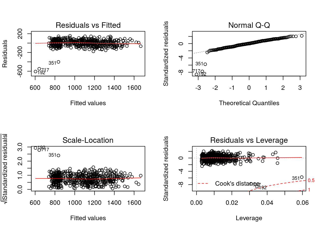
There is some indication of non-normality seen in the Normal Q-Q plot and the presence of outliers in the Residuals vs Leverage plot are consistent with the fact that this model is misspecified.
The methods discussed in this chapter use the backward iterative algorithm to obtain parameter estimates for the Q-function models. Thus, the pseudo-outcome is used in the second stage regression that follows. Recall, the pseudo-outcome at this decision point is an individuals expected outcome had they received treatment according the optimal treatment regime at Decision 3. The optimal regime is that which maximizes the Q-function, and thus we calculate the pseudo-outcome as follows. Notice that for individuals that received \(A_{2} = 1\), the pseudo-outcome is taken to be the final response .
A3 <- dataMDPF$A3
dataMDPF$A3 <- 0L
Q30 <- stats::predict(object = Q3, newdata = dataMDPF[!oneA3,])
dataMDPF$A3 <- 1L
Q31 <- stats::predict(object = Q3, newdata = dataMDPF[!oneA3,])
dataMDPF$A3 <- A3
V3 <- dataMDPF$Y
V3[!oneA3] <- pmax(Q30, Q31)The posited model for \(Q_{2}(h_{2},a_{2}) = E\{V_{3}(H_{3})|H_{2} = h_{2}, A_{2} = a_{2}\}\) is misspecified as
\[ Q_{2}(h_{2},a_{2};\beta_{2}) = \beta_{20} + \beta_{21} \text{CD4_0} + \beta_{22} \text{CD4_6} + a_{2}~(\beta_{23} + \beta_{24} \text{CD4_6}). \]
Modeling Object
The parameters of this model will be estimated using ordinary least squares via
The modeling objects for this regression step is
q2 <- modelObj::buildModelObj(model = ~ CD4_0 + CD4_6*A2,
                              solver.method = 'lm',
predict.method = 'predict.lm')Model Diagnostics
Recall that individuals for whom only one treatment option is available should not be included in the regression analysis; i.e., individuals that received treatment \(A_{1} = 1\) remained on treatment 1 at the second stage.
oneA2 <- dataMDPF$A1 == 1LThe pseudo-outcome, \(V_{3}(H_{3})\), was calculated under the previous tab. For \(Q_{2}(h_{2},a_{2};{\beta}_{2})\) the regression can be completed as follows
Q2 <- modelObj::fit(object = q2,
data = dataMDPF[!oneA2,],
response = V3[!oneA2])
Q2 <- modelObj::fitObject(object = Q2)
Q2
Call:
lm(formula = YinternalY ~ CD4_0 + CD4_6 + A2 + CD4_6:A2, data = data)
Coefficients:
(Intercept) CD4_0 CD4_6 A2 CD4_6:A2
344.9733 1.8566 -0.1238 500.7085 -1.6028 where for convenience we have again made use of modelObj’s
In examining the diagnostic plots defined for “lm” objects
par(mfrow = c(2,2))
graphics::plot(x = Q2)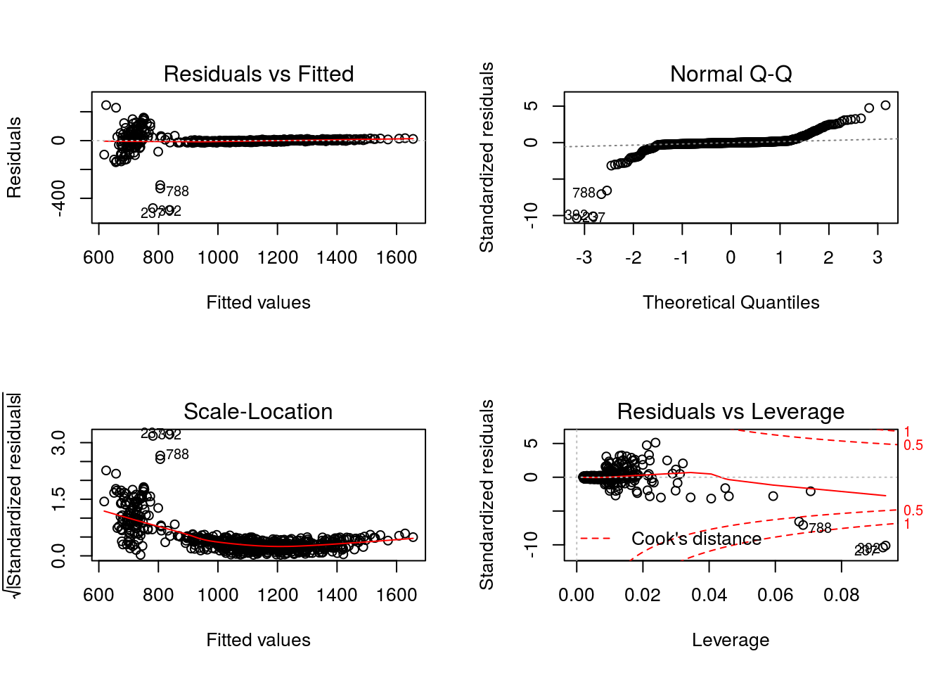
The non-normality of the residuals is consistent with the fact that this model is misspecified.
The methods discussed in this chapter use the backward iterative algorithm to obtain parameter estimates for the Q-function models. Thus, the pseudo-outcome is used in the first stage regression that follows. Recall, the pseudo-outcome at this decision point is an individuals expected outcome had they received treatment according the optimal treatment regime at Decisions 2 and 3. The optimal regime is that which maximizes the Q-function, and thus we calculate the pseudo-outcome as follows. Note that for individuals that received \(A_{1} = 1\) and were thus not included in the model fitting procedure, the pseudo-outcome is equal to the Decision 3 pseudo-outcome.
A2 <- dataMDPF$A2
dataMDPF$A2 <- 0L
Q20 <- stats::predict(object = Q2, newdata = dataMDPF[!oneA2,])
dataMDPF$A2 <- 1L
Q21 <- stats::predict(object = Q2, newdata = dataMDPF[!oneA2,])
dataMDPF$A2 <- A2
V2 <- V3
V2[!oneA2] <- pmax(Q20, Q21)The posited model for \(Q_{1}(h_{1},a_{1}) = E\{V_{2}(H_{2})|H_{1} = h_{1}, A_{1} = a_{1}\}\) is taken to be
\[ Q_{1}(h_{1},a_{1};\beta_{1}) = \beta_{10} + \beta_{11} \text{CD4_0} + a_{1}~(\beta_{12} + \beta_{13} \text{CD4_0}). \]
Modeling Object
The parameters of this model will be estimated using ordinary least squares via
The modeling objects for this regression step is
q1 <- modelObj::buildModelObj(model = ~ CD4_0*A1,
                              solver.method = 'lm',
predict.method = 'predict.lm')Model Diagnostics
Recall that \(Q_{1}(h_{1},a_{1})\) is the expectation of the value, \(V_{2}(H_{2})\); we use the results discussed in the previous regression analysis. For \(Q_{1}(h_{1},a_{1};\beta_{1})\) the regression can be completed as follows
Q1 <- modelObj::fit(object = q1, data = dataMDPF, response = V2)
Q1 <- modelObj::fitObject(object = Q1)
Q1
Call:
lm(formula = YinternalY ~ CD4_0 + A1 + CD4_0:A1, data = data)
Coefficients:
(Intercept) CD4_0 A1 CD4_0:A1
379.564 1.632 477.623 -1.932 where for convenience we have again made use of modelObj’s
In examining the diagnostic plots defined for “lm” objects
par(mfrow = c(2,2))
graphics::plot(x = Q1)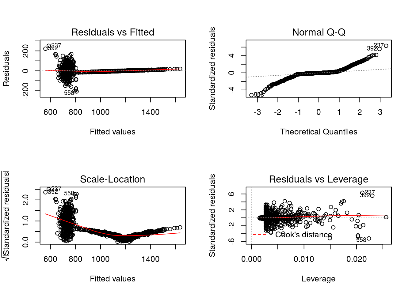
The non-normality seen in the Normal Q-Q plot and the presence of outliers in the Residuals vs Leverage plot are consistent with the fact that this model is misspecified.
\(\omega_{k}(h_{k},a_{k};\gamma_{k })\)
For Chapters 6 and 7, we consider a single model for each of the three propensity scores. It is not our objective to demonstrate a definitive analysis that one might do in practice but to illustrate how to apply the methods. The posited models are intentionally kept simple and likely to be familiar to most readers. By this, we avoid adding any additional complexity to the discussion. In practice, analysist would perform model and variable selection techniques, etc., to arrive at a posited model.
Click on each tab below to see the model and basic model diagnostic steps.
The posited model for the first decision point is the model used to generate the data
\[ \omega_{1}(h_{1},1;\gamma_{1}) = \frac{\exp(\gamma_{10} + \gamma_{11}~\text{CD4_0})}{1+\exp(\gamma_{10} + \gamma_{11}~\text{CD4_0})}. \]
Modeling Object
The parameters of this model will be estimated using maximum likelihood via
p1 <- modelObj::buildModelObj(model = ~ CD4_0,
                              solver.method = 'glm',
                              solver.args = list(family='binomial'),
                              predict.method = 'predict.glm',
predict.args = list(type='response'))Model Diagnostics
For \(\omega_{1}(h_{1},1;\gamma_{1})\) the regression can be completed as follows:
PS1 <- modelObj::fit(object = p1, data = dataMDPF, response = dataMDPF$A1)
PS1 <- modelObj::fitObject(object = PS1)
PS1
Call: glm(formula = YinternalY ~ CD4_0, family = "binomial", data = data)
Coefficients:
(Intercept) CD4_0
2.385956 -0.006661
Degrees of Freedom: 999 Total (i.e. Null); 998 Residual
Null Deviance: 1316
Residual Deviance: 1227 AIC: 1231where for convenience we have made use of modelObj’s
Though we know this model to be correctly specified, let’s examine the regression results.
summary(object = PS1)
Call:
glm(formula = YinternalY ~ CD4_0, family = "binomial", data = data)
Deviance Residuals:
Min 1Q Median 3Q Max
-1.9111 -0.9416 -0.7097 1.2143 2.1092
Coefficients:
Estimate Std. Error z value Pr(>|z|)
(Intercept) 2.3859559 0.3359581 7.102 1.23e-12 ***
CD4_0 -0.0066608 0.0007601 -8.763 < 2e-16 ***
---
Signif. codes: 0 '***' 0.001 '**' 0.01 '*' 0.05 '.' 0.1 ' ' 1
(Dispersion parameter for binomial family taken to be 1)
Null deviance: 1315.8 on 999 degrees of freedom
Residual deviance: 1227.3 on 998 degrees of freedom
AIC: 1231.3
Number of Fisher Scoring iterations: 4In comparing the null deviance (1315.8) and the residual deviance (1227.3), we see that including the independent variable, \(\text{CD4_0}\) does reduce the deviance. This result is consistent with the fact that it is the model used to generate the data.
The posited model for the second decision point is the model used to generate the data for individuals in subset \(s_{2}(h_{2}) = 2\), for whom more than one treatment option was available
\[ \omega_{2,2}(h_{2},1;\gamma_{2}) = \frac{\exp(\gamma_{20} + \gamma_{21}~\text{CD4_6})}{1+\exp(\gamma_{20} + \gamma_{21}~\text{CD4_6})}. \]
Modeling Object
The parameters of this model will be estimated using maximum likelihood via
p2 <- modelObj::buildModelObj(model = ~ CD4_6,
                              solver.method = 'glm',
                              solver.args = list(family='binomial'),
                              predict.method = 'predict.glm',
predict.args = list(type='response'))Model Diagnostics
Recall that individuals for whom only one treatment option is available should not be included in the regression analysis; i.e., individuals that received treatment \(A_{1} = 1\) received treatment \(A_{2} = 1\) with probability 1.
oneA2 <- dataMDPF$A1 == 1LFor \(\omega_{2,2}(h_{2},1;\gamma_{2})\) the regression can be completed as follows:
PS2 <- modelObj::fit(object = p2,
data = dataMDPF[!oneA2,],
response = dataMDPF$A2[!oneA2])
PS2 <- modelObj::fitObject(object = PS2)
PS2
Call: glm(formula = YinternalY ~ CD4_6, family = "binomial", data = data)
Coefficients:
(Intercept) CD4_6
1.234491 -0.004781
Degrees of Freedom: 631 Total (i.e. Null); 630 Residual
Null Deviance: 608.5
Residual Deviance: 577.8 AIC: 581.8where for convenience we have made use of modelObj’s
Though we know this model to be correctly specified, let’s examine the regression results.
summary(object = PS2)
Call:
glm(formula = YinternalY ~ CD4_6, family = "binomial", data = data)
Deviance Residuals:
Min 1Q Median 3Q Max
-1.2815 -0.6751 -0.5572 -0.4062 2.4387
Coefficients:
Estimate Std. Error z value Pr(>|z|)
(Intercept) 1.2344914 0.5042630 2.448 0.0144 *
CD4_6 -0.0047811 0.0009013 -5.304 1.13e-07 ***
---
Signif. codes: 0 '***' 0.001 '**' 0.01 '*' 0.05 '.' 0.1 ' ' 1
(Dispersion parameter for binomial family taken to be 1)
Null deviance: 608.51 on 631 degrees of freedom
Residual deviance: 577.83 on 630 degrees of freedom
AIC: 581.83
Number of Fisher Scoring iterations: 4In comparing the null deviance (608.5) and the residual deviance (577.8), we see that including the independent variable, \(\text{CD4_6}\) reduces the deviance. This result is consistent with the fact that it is the model used to generate the data.
The posited model for the final decision point is the model used to generate the data for individuals in subset \(s_{3}(h_{3}) = 2\), for whom more than one treatment option was available
\[ \omega_{3,2}(h_{3},1;\gamma_{3}) = \frac{\exp(\gamma_{30} + \gamma_{31}~\text{CD4_12})}{1+\exp(\gamma_{30} + \gamma_{31}~\text{CD4_12})}. \]
Modeling Object
The parameters of this model will be estimated using maximum likelihood via
p3 <- modelObj::buildModelObj(model = ~ CD4_12,
                              solver.method = 'glm',
                              solver.args = list(family='binomial'),
                              predict.method = 'predict.glm',
predict.args = list(type='response'))Model Diagnostics
Recall that individuals for whom only one treatment option is available should not be included in the regression analysis; i.e., individuals that received treatment \(A_{2} = 1\) were assigned treatment \(A_{3} = 1\) with probability 1.
oneA3 <- dataMDPF$A2 == 1LFor \(\omega_{3,2}(h_{3},1;\gamma_{3})\) the regression can be completed as follows:
PS3 <- modelObj::fit(object = p3,
                     data = dataMDPF[!oneA3,],
                     response = dataMDPF$A3[!oneA3])
PS3 <- modelObj::fitObject(object = PS3)
PS3
Call:  glm(formula = YinternalY ~ CD4_12, family = "binomial", data = data)

Coefficients:
(Intercept)       CD4_12
   0.929409    -0.003816

Degrees of Freedom: 513 Total (i.e. Null);  512 Residual
Null Deviance:      622.5
Residual Deviance: 609.1    AIC: 613.1
where for convenience we have made use of modelObj’s
Though we know this model to be correctly specified, let’s examine the regression results.
summary(object = PS3)
Call:
glm(formula = YinternalY ~ CD4_12, family = "binomial", data = data)

Deviance Residuals:
    Min       1Q   Median       3Q      Max
-1.2985  -0.8629  -0.7505   1.3664   1.8875

Coefficients:
             Estimate Std. Error z value Pr(>|z|)
(Intercept)  0.929409   0.508608   1.827 0.067646 .
CD4_12      -0.003816   0.001069  -3.569 0.000359 ***
---
Signif. codes:  0 '***' 0.001 '**' 0.01 '*' 0.05 '.' 0.1 ' ' 1

(Dispersion parameter for binomial family taken to be 1)

    Null deviance: 622.45  on 513  degrees of freedom
Residual deviance: 609.14  on 512  degrees of freedom
AIC: 613.14

Number of Fisher Scoring iterations: 4
In comparing the null deviance (622.5) and the residual deviance (609.1), we see that including the independent variable, \(\text{CD4_12}\) reduces the deviance. This result is consistent with the fact that it is the model used to generate the data.