
Classification Estimator
The classification estimator is obtained by minimizing in \(\eta_{1}\)
\[ \begin{align} n^{-1} \sum_{i=1}^{n} \left| \widehat{C}_1(H_{1i}, A_{1i}, Y_i) \right|~ \text{I}\Big[ \text{I}\left\{\widehat{C}_1(H_{1i}, A_{1i}, Y_i) \geq 0 \right\} \neq \text{I}\{ d_{1}(H_{1i}; \eta_{1}) = 1\}\Big], \end{align} \]
where \(\widehat{C}_{1}(H_{1i},A_{1i},Y_{i})\) is termed the contrast function defined as
\[ \widehat{C}_{1}(H_{1i},A_{1i},Y_{i}) = \widehat{\psi}_{1}(H_{1i}, A_{1i}, Y_{i}) - \widehat{\psi}_{0}(H_{1i}, A_{1i}, Y_{i}). \]
For the augmented inverse probability weighted value estimator,
\[ \begin{align} \psi_{1}(H_{1}, A_{1}, Y) = \frac{ A_{1}}{\pi_{1}(H_{1}) } Y_{i} - \frac{\{A_{1} - \pi_{1}(H_{1}) \} }{\pi_{1}(H_{1}) }Q_{1}(H_{1},1) \quad \quad \text{and} \end{align} \] \[ \begin{align} \psi_{0}(H_{1}, A_{1}, Y) = \frac{ 1 - A_{1}}{1 - \pi_{1}(H_{1}) } Y_{i} - \frac{A_{1} - \pi_{1}(H_{1}) }{1 - \pi_{1}(H_{1}) }Q_{1}(H_{1},0), \end{align} \] where \(Q_{1}(h_{1},a_{1}) = E(Y|H_{1}=h_{1},A_{1} = a_{1})\) and \(\pi_{1}(h_{1}) = P(A_{1} = 1|H_{1} = h_{1})\). The estimator \(\widehat{\psi}_{a_{1}}(H_{1i}, A_{1i}, Y_{i})\) is \(\psi_{a_{1}}(H_{1}, A_{1}, Y)\) evaluated at \((H_{1i}, A_{1i}, Y_{i})\) with fitted models \(Q_{1}(h_{1}, a_{1};\widehat{\beta}_{1})\) and \(\pi_{1}(h_{1};\widehat{\gamma}_{1})\) substituted for \(Q_{1}(h_{1}, a_{1})\) and \(\pi_{1}(h_{1})\), respectively.
Comparison of the expression to be minimized to the standard weighted classification error of the generic classification problem shows that \(\left| \widehat{C}_1(H_{1i}, A_{1i}, Y_i)\right|\) can be identified as the “weight”, \(\text{I}\{ \widehat{C}_1(H_{1i}, A_{1i}, Y_i) \geq 0\}\) as the “label,” and \(\text{I}\{ d_{1}(H_{1i}; \eta_{1}) = 1\}\) as the “classifier.” There are numerous methods available for solving the weighted classification problem.
The simple inverse probability weighted estimator, \(\widehat{\mathcal{V}}_{IPW}(d_{\eta})\), is the special case of \(\widehat{\mathcal{V}}_{AIPW}(d_{\eta})\) when \(Q_{1}(h_{1},a_{1}) \equiv 0\).
The simple and augmented inverse probability weighted classification estimator is implemented as
The function call for DynTxRegime::
utils::str(object = DynTxRegime::optimalClass)function (..., moPropen, moMain, moCont, moClass, data, response, txName, iter = 0L, fSet = NULL, verbose = TRUE) We briefly describe the input arguments for DynTxRegime::
| Input Argument | Description |
|---|---|
| \(\dots\) | Ignored; included only to require named inputs. |
| moPropen | A “modelObj” object. The modeling object for the propensity score regression step. |
| moMain | A “modelObj” object. The modeling object for the \(\nu_{1}(h_{1}; \phi_{1})\) component of \(Q_{1}(h_{1},a_{1};\beta_{1})\). |
| moCont | A “modelObj” object. The modeling object for the \(\text{C}_{1}(h_{1}; \psi_{1})\) component of \(Q_{1}(h_{1},a_{1};\beta_{1})\). |
| moClass | A “modelObj” object. The modeling object for the classification regression step. |
| data | A “data.frame” object. The covariate history and the treatment received. |
| response | A “numeric” vector. The outcome of interest, where larger values are better. |
| txName | A “character” object. The column header of data corresponding to the treatment variable. |
| iter | An “integer” object. The maximum number of iterations for iterative algorithm. |
| fSet | A “function”. A user defined function specifying treatment or model subset structure. |
| verbose | A “logical” object. If TRUE progress information is printed to screen. |
Methods implemented in DynTxRegime break the outcome model into two components: a main effects component and a contrasts component. For example, for binary treatments, \(Q_{1}(h_{1}, a_{1}; \beta_{1})\) can be written as
\[ Q_{1}(h_{1}, a_{1}; \beta_{1})= \nu_{1}(h_{1}; \phi_{1}) + a_{1} \text{C}_{1}(h_{1}; \psi_{1}), \]
where \(\beta_{1} = (\phi^{\intercal}_{1}, \psi^{\intercal}_{1})^{\intercal}\). Here, \(\nu_{1}(h_{1}; \phi_{1})\) comprises the terms of the outcome regression model that are independent of treatment (so called “main effects” or “common effects”), and \(\text{C}_{1}(h_{1}; \psi_{1})\) comprises the terms of the model that interact with treatment (so called “contrasts”). Input arguments moMain and moCont specify \(\nu_{1}(h_{1}; \phi_{1})\) and \(\text{C}_{1}(h_{1}; \psi_{1})\), respectively.
In the examples provided in this chapter, the two components of \(Q_{1}(h_{1}, a_{1}; \beta_{1})\) are both linear models, the parameters of which are estimated using stats::
The value object returned by DynTxRegime::
| Slot Name | Description |
|---|---|
| @step | For single decision analyses this will always be 1. |
| @analysis@classif | The classification results. |
| @analysis@outcome | The outcome regression analysis if AIPW value estimator; NA otherwise. |
| @analysis@propen | The propensity score regression analysis. |
| @analysis@call | The unevaluated function call. |
| @analysis@optimal | The estimated value and optimal treatment for the training data. |
There are several methods available for objects of this class that assist with model diagnostics, the exploration of training set results, and the estimation of optimal treatments for future patients. We explore these methods under the Methods tabs.
We continue to consider the outcome regression and propensity score models introduced in Chapter 2, which represent a range of model (mis)specification. For brevity, we discuss the function call to DynTxRegime::
Input moPropen is a modeling object for the propensity score regression. To illustrate the function call, we will use the true propensity score model
\[ \pi^{3}_{1}(h_{1};\gamma_{1}) = \frac{\exp(\gamma_{10} + \gamma_{11}~\text{SBP0} + \gamma_{12}~\text{Ch})}{1+\exp(\gamma_{10} + \gamma_{11}~\text{SBP0}+ \gamma_{12}~\text{Ch})}, \] which is defined as a modeling object as follows
p3 <- modelObj::buildModelObj(model = ~ SBP0 + Ch,
                              solver.method = 'glm',
                              solver.args = list(family='binomial'),
                              predict.method = 'predict.glm',
predict.args = list(type='response'))For the augmented inverse probability weighted value estimator, moMain and moCont are modeling objects specifying the outcome regression. To illustrate, we will use the true outcome regression model
\[ Q^{3}_{1}(h_{1},a_{1};\beta_{1}) = \beta_{10} + \beta_{11} \text{Ch} + \beta_{12} \text{K} + a_{1}~(\beta_{13} + \beta_{14} \text{Ch} + \beta_{15} \text{K}), \]
which is defined as modeling objects as follows
q3Main <- modelObj::buildModelObj(model = ~ (Ch + K),
                                  solver.method = 'lm',
                                  predict.method = 'predict.lm')
q3Cont <- modelObj::buildModelObj(model = ~ (Ch + K),
solver.method = 'lm',
predict.method = 'predict.lm')Note that the formula in the contrast component does not contain the treatment variable; it contains only the covariates that interact with the treatment.
Both components of the outcome regression model are of the same class, and the models for each decision point should be fit as a single combined object. Thus, the iterative algorithm is not required, and iter should keep its default value.
For the inverse probability weighted value estimator, moMain and moCont are NULL.
Input moClass is a modeling object that specifies the restricted class of regimes and the
library(rpart)
moC <- modelObj::buildModelObj(model = ~ W + K + Cr + Ch,
                               solver.method = 'rpart',
                               predict.args = list(type='class'))
Notice that we have modified the default prediction arguments, predict.args, to ensure that predictions are returned as the class to which the record is assigned. For this method, predictions for the classification step must be the assigned class.
As for all methods discussed in this chapter: the “data.frame” containing the baseline covariates and treatment received is data set dataSBP, the treatment is contained in column $A of dataSBP, and the outcome of interest is the change in systolic blood pressure measured six months after treatment, \(y = \text{SBP0} - \text{SBP6}\), which is already defined in our R environment.
The optimal treatment regime is estimated as follows.
AIPW33 <- DynTxRegime::optimalClass(moPropen = p3,
                                    moMain = q3Main,
                                    moCont = q3Cont,
                                    moClass = moC,
                                    data = dataSBP,
                                    response = y,
                                    txName = 'A',
                                    verbose = TRUE)
AIPW value estimator
First step of the Classification Algorithm.
Classification Perspective.
Propensity for treatment regression.
Regression analysis for moPropen:
Call: glm(formula = YinternalY ~ SBP0 + Ch, family = "binomial", data = data)
Coefficients:
(Intercept) SBP0 Ch
-15.94153 0.07669 0.01589
Degrees of Freedom: 999 Total (i.e. Null); 997 Residual
Null Deviance: 1378
Residual Deviance: 1162 AIC: 1168
Outcome regression.
Combined outcome regression model: ~ Ch+K + A + A:(Ch+K) .
Regression analysis for Combined:
Call:
lm(formula = YinternalY ~ Ch + K + A + Ch:A + K:A, data = data)
Coefficients:
(Intercept) Ch K A Ch:A K:A
-15.6048 -0.2035 12.2849 -61.0979 0.5048 -6.6099
Classification Analysis
Regression analysis for moClass:
n= 1000

node), split, n, loss, yval, (yprob)
      * denotes terminal node

 1) root 1000 0.1401350000 1 (0.025873081 0.974126919)
   2) Ch< 183.55 285 0.0166130600 0 (0.568407075 0.431592925)
     4) Ch< 155.2 119 0.0017551050 0 (0.905908559 0.094091441) *
     5) Ch>=155.2 166 0.0148579600 0 (0.251082865 0.748917135)
      10) K>=4.25 80 0.0026340590 0 (0.552429068 0.447570932) *
      11) K< 4.25 86 0.0106160000 1 (0.123987442 0.876012558)
        22) W< 62.9 21 0.0012200790 0 (0.373747901 0.626252099) *
        23) W>=62.9 65 0.0061481210 1 (0.083457937 0.916542063)
          46) Cr< 0.75 19 0.0009908188 0 (0.315338047 0.684661953) *
          47) Cr>=0.75 46 0.0033479920 1 (0.051676480 0.948323520) *
   3) Ch>=183.55 715 0.0058836740 1 (0.001135832 0.998864168) *
Recommended Treatments:
0 1
239 761
Estimated value: 13.23713 Above, we opted to set verbose to TRUE to highlight some of the information that should be verified by a user. Notice the following:
- The first few lines of the verbose output indicates that the selected value estimator is the augmented inverse probability weighted estimator from the classification perspective. Users can also use this function for multiple decision point settings, which is why users are informed that this is the “First step of the Classification Algorithm”.
Users should verify that this is the intended estimator and correct step. - The information provided for the propensity score, outcome, and classification regressions is not defined within DynTxRegime::
optimalSeq() , but is specified by the statistical methods selected to obtain parameter estimates; in this example it is defined by stats::glm() , stats::lm() , rpart::rpart() , respectively.
Users should verify that the models were correctly interpreted by the software and that there are no warnings or messages reported by the regression methods. - Finally, a tabled summary of the recommended treatments and the estimated value for the training data are shown. The sum of the elements of the table should be the number of individuals in the training data. If it is not, the data set is likely not complete; method implementation in DynTxRegime require complete data sets.
The first step of the post-analysis should always be model diagnostics. DynTxRegime comes with several tools to assist in this task. However, we have explored the outcome regression models previously and will skip that step here. Available model diagnostic tools are described under the Methods tab.
The estimated optimal treatment regime can be retrieved using DynTxRegime::
DynTxRegime::classif(object = AIPW33)n= 1000
node), split, n, loss, yval, (yprob)
* denotes terminal node
1) root 1000 0.1401350000 1 (0.025873081 0.974126919)
2) Ch< 183.55 285 0.0166130600 0 (0.568407075 0.431592925)
4) Ch< 155.2 119 0.0017551050 0 (0.905908559 0.094091441) *
5) Ch>=155.2 166 0.0148579600 0 (0.251082865 0.748917135)
10) K>=4.25 80 0.0026340590 0 (0.552429068 0.447570932) *
11) K< 4.25 86 0.0106160000 1 (0.123987442 0.876012558)
22) W< 62.9 21 0.0012200790 0 (0.373747901 0.626252099) *
23) W>=62.9 65 0.0061481210 1 (0.083457937 0.916542063)
46) Cr< 0.75 19 0.0009908188 0 (0.315338047 0.684661953) *
47) Cr>=0.75 46 0.0033479920 1 (0.051676480 0.948323520) *
3) Ch>=183.55 715 0.0058836740 1 (0.001135832 0.998864168) *The structure of the returned object is defined by the classification method specified. For rpart::
There are several methods available for the returned object that assist with model diagnostics, the exploration of training set results, and the estimation of optimal treatments for future patients. A complete description of these methods can be found under the Methods tab.
In the table below, we show the estimated value obtained using the simple and augmented inverse weighted value estimators obtained from the classification perspective. For the simple inverse probability weighted estimator, we show results under each of the propensity score models considered; for the augmented inverse probability weighted estimator, we show results for all combinations of outcome and propensity score models.
| (mmHG) | \(Q^{1}_{1}(h_{1},a_{1};\beta_{1})\) | \(Q^{2}_{1}(h_{1},a_{1};\beta_{1})\) | \(Q^{3}_{1}(h_{1},a_{1};\beta_{1})\) | |
| \(\pi^{1}_{1}(h_{1};\gamma_{1})\) | 16.96 | 16.06 | 13.17 | 13.08 |
| \(\pi^{2}_{1}(h_{1};\gamma_{1})\) | 13.18 | 13.32 | 13.10 | 13.09 |
| \(\pi^{3}_{1}(h_{1};\gamma_{1})\) | 13.10 | 13.79 | 13.22 | 13.24 |
For the same conditions as described above, below we show the number of individuals recommended to each treatment option.
| \((n_{\widehat{d} = 0},n_{\widehat{d} = 1})\) | \(Q^{1}_{1}(h_{1},a_{1};\beta_{1})\) | \(Q^{2}_{1}(h_{1},a_{1};\beta_{1})\) | \(Q^{3}_{1}(h_{1},a_{1};\beta_{1})\) | |
| \(\pi^{1}_{1}(h_{1};\gamma_{1})\) | (232, 768) | (132, 868) | (226, 774) | (248, 752) |
| \(\pi^{2}_{1}(h_{1};\gamma_{1})\) | (269, 731) | (239, 761) | (258, 742) | (248, 752) |
| \(\pi^{3}_{1}(h_{1};\gamma_{1})\) | (239, 761) | (184, 816) | (239, 761) | (239, 761) |
We illustrate the methods available for objects of class “OptimalClass” by considering the following analysis:
p3 <- modelObj::buildModelObj(model = ~ SBP0 + Ch,
                              solver.method = 'glm',
                              solver.args = list(family='binomial'),
                              predict.method = 'predict.glm',
                              predict.args = list(type='response'))
q3Main <- modelObj::buildModelObj(model = ~ (Ch + K),
solver.method = 'lm',
predict.method = 'predict.lm')q3Cont <- modelObj::buildModelObj(model = ~ (Ch + K),
solver.method = 'lm',
predict.method = 'predict.lm')library(rpart)
moC <- modelObj::buildModelObj(model = ~ W + K + Cr + Ch,
solver.method = 'rpart',
predict.args = list(type='class'))result <- DynTxRegime::optimalClass(moPropen = p3,
moMain = q3Main,
moCont = q3Cont,
moClass = moC,
data = dataSBP,
response = y,
txName = 'A',
verbose = FALSE)| Function | Description |
|---|---|
| Call(name, …) | Retrieve the unevaluated call to the statistical method. |
| classif(object, …) | Retrieve the regression analysis for the classification step. |
| coef(object, …) | Retrieve estimated parameters of postulated propensity and/or outcome models. |
| DTRstep(object) | Print description of method used to estimate the treatment regime and value. |
| estimator(x, …) | Retrieve the estimated value of the estimated optimal treatment regime for the training data set. |
| fitObject(object, …) | Retrieve the regression analysis object(s) without the modelObj framework. |
| optTx(x, …) | Retrieve the estimated optimal treatment regime and decision functions for the training data. |
| optTx(x, newdata, …) | Predict the optimal treatment regime for new patient(s). |
| outcome(object, …) | Retrieve the regression analysis for the outcome regression step. |
| plot(x, suppress = FALSE, …) | Generate diagnostic plots for the regression object (input suppress = TRUE suppresses title changes indicating regression step.). |
| print(x, …) | Print main results. |
| propen(object, …) | Retrieve the regression analysis for the propensity score regression step |
| show(object) | Show main results. |
| summary(object, …) | Retrieve summary information from regression analyses. |
The unevaluated call to the statistical method can be retrieved as follows
DynTxRegime::Call(name = result)DynTxRegime::optimalClass(moPropen = p3, moMain = q3Main, moCont = q3Cont,
moClass = moC, data = dataSBP, response = y, txName = "A",
verbose = FALSE)The returned object can be used to re-call the analysis with modified inputs.
For example, to complete the analysis with a different classification model requires only the following code.
moC <- modelObj::buildModelObj(model = ~ W + K + Ch,
solver.method = 'rpart',
solver.args = list("control"=list("maxdepth"=1)),
predict.args = list(type='class'))
result_c2 <- eval(expr = DynTxRegime::Call(name = result))This function provides a reminder of the analysis used to obtain the object.
DynTxRegime::DTRstep(object = result)Classification Perspective - Step 1 The
DynTxRegime::summary(object = result)Call:
rpart(formula = YinternalY ~ W + K + Cr + Ch, data = data, weights = wgt)
n= 1000
CP nsplit rel error xerror xstd
1 0.83946381 0 1.0000000 1.0000000 2.477090
2 0.01155005 1 0.1605362 0.1828370 1.127515
3 0.01000000 5 0.1129748 0.1819606 1.124881
Variable importance
Ch K W Cr
96 3 1 1
Node number 1: 1000 observations, complexity param=0.8394638
predicted class=1 expected loss=0.140135 P(node) =1
class counts: 0.140135 0.859865
probabilities: 0.026 0.974
left son=2 (285 obs) right son=3 (715 obs)
Primary splits:
Ch < 183.55 to the left, improve=0.1997412000, (0 missing)
K < 4.55 to the right, improve=0.0037713730, (0 missing)
W < 51.15 to the right, improve=0.0008306307, (0 missing)
Cr < 0.65 to the right, improve=0.0004318633, (0 missing)
Surrogate splits:
K < 3.3 to the left, agree=0.850, adj=0.007, (0 split)
W < 40.6 to the left, agree=0.849, adj=0.001, (0 split)
Node number 2: 285 observations, complexity param=0.01155005
predicted class=0 expected loss=0.1101192 P(node) =0.1508644
class counts: 0.134251 0.0166131
probabilities: 0.568 0.432
left son=4 (119 obs) right son=5 (166 obs)
Primary splits:
Ch < 155.2 to the left, improve=6.119716e-03, (0 missing)
K < 4.25 to the right, improve=1.401295e-03, (0 missing)
W < 64.15 to the left, improve=2.313978e-04, (0 missing)
Cr < 0.65 to the right, improve=8.605709e-05, (0 missing)
Surrogate splits:
Cr < 0.65 to the right, agree=0.712, adj=0.042, (0 split)
W < 110.4 to the left, agree=0.702, adj=0.010, (0 split)
K < 3.3 to the right, agree=0.699, adj=0.001, (0 split)
Node number 3: 715 observations
predicted class=1 expected loss=0.006929016 P(node) =0.8491356
class counts: 0.00588367 0.843252
probabilities: 0.001 0.999
Node number 4: 119 observations
predicted class=0 expected loss=0.01664532 P(node) =0.1054413
class counts: 0.103686 0.0017551
probabilities: 0.906 0.094
Node number 5: 166 observations, complexity param=0.01155005
predicted class=0 expected loss=0.3271015 P(node) =0.04542308
class counts: 0.0305651 0.014858
probabilities: 0.251 0.749
left son=10 (80 obs) right son=11 (86 obs)
Primary splits:
K < 4.25 to the right, improve=0.0039787890, (0 missing)
Ch < 174.45 to the left, improve=0.0016532860, (0 missing)
Cr < 0.75 to the left, improve=0.0010648220, (0 missing)
W < 64.1 to the left, improve=0.0003872463, (0 missing)
Surrogate splits:
Ch < 160.55 to the left, agree=0.600, adj=0.196, (0 split)
W < 83.7 to the left, agree=0.548, adj=0.090, (0 split)
Cr < 0.75 to the left, agree=0.530, adj=0.054, (0 split)
Node number 10: 80 observations
predicted class=0 expected loss=0.1166381 P(node) =0.02258318
class counts: 0.0199491 0.00263406
probabilities: 0.552 0.448
Node number 11: 86 observations, complexity param=0.01155005
predicted class=1 expected loss=0.4648006 P(node) =0.0228399
class counts: 0.010616 0.0122239
probabilities: 0.124 0.876
left son=22 (21 obs) right son=23 (65 obs)
Primary splits:
W < 62.9 to the left, improve=0.0015579640, (0 missing)
Cr < 0.75 to the left, improve=0.0008539991, (0 missing)
Ch < 179.25 to the left, improve=0.0005386285, (0 missing)
K < 3.55 to the right, improve=0.0004120074, (0 missing)
Surrogate splits:
Ch < 181.5 to the right, agree=0.759, adj=0.031, (0 split)
Node number 22: 21 observations
predicted class=0 expected loss=0.2145022 P(node) =0.005687955
class counts: 0.00446788 0.00122008
probabilities: 0.374 0.626
Node number 23: 65 observations, complexity param=0.01155005
predicted class=1 expected loss=0.3584505 P(node) =0.01715194
class counts: 0.00614812 0.0110038
probabilities: 0.083 0.917
left son=46 (19 obs) right son=47 (46 obs)
Primary splits:
Cr < 0.75 to the left, improve=1.406834e-03, (0 missing)
Ch < 180.3 to the left, improve=7.245144e-04, (0 missing)
W < 66.45 to the right, improve=3.038534e-04, (0 missing)
K < 3.95 to the left, improve=2.129029e-05, (0 missing)
Surrogate splits:
W < 63.75 to the left, agree=0.789, adj=0.044, (0 split)
Node number 46: 19 observations
predicted class=0 expected loss=0.2613644 P(node) =0.003790948
class counts: 0.00280013 0.000990819
probabilities: 0.315 0.685
Node number 47: 46 observations
predicted class=1 expected loss=0.2505796 P(node) =0.01336099
class counts: 0.00334799 0.010013
probabilities: 0.052 0.948 $propensity
Call:
glm(formula = YinternalY ~ SBP0 + Ch, family = "binomial", data = data)
Deviance Residuals:
Min 1Q Median 3Q Max
-2.3891 -0.9502 -0.4940 0.9939 2.1427
Coefficients:
Estimate Std. Error z value Pr(>|z|)
(Intercept) -15.941527 1.299952 -12.263 <2e-16 ***
SBP0 0.076687 0.007196 10.657 <2e-16 ***
Ch 0.015892 0.001753 9.066 <2e-16 ***
---
Signif. codes: 0 '***' 0.001 '**' 0.01 '*' 0.05 '.' 0.1 ' ' 1
(Dispersion parameter for binomial family taken to be 1)
Null deviance: 1377.8 on 999 degrees of freedom
Residual deviance: 1161.6 on 997 degrees of freedom
AIC: 1167.6
Number of Fisher Scoring iterations: 3
$outcome
$outcome$Combined
Call:
lm(formula = YinternalY ~ Ch + K + A + Ch:A + K:A, data = data)
Residuals:
Min 1Q Median 3Q Max
-9.0371 -1.9376 0.0051 2.0127 9.6452
Coefficients:
Estimate Std. Error t value Pr(>|t|)
(Intercept) -15.604845 1.636349 -9.536 <2e-16 ***
Ch -0.203472 0.002987 -68.116 <2e-16 ***
K 12.284852 0.358393 34.278 <2e-16 ***
A -61.097909 2.456637 -24.871 <2e-16 ***
Ch:A 0.504816 0.004422 114.168 <2e-16 ***
K:A -6.609876 0.538386 -12.277 <2e-16 ***
---
Signif. codes: 0 '***' 0.001 '**' 0.01 '*' 0.05 '.' 0.1 ' ' 1
Residual standard error: 2.925 on 994 degrees of freedom
Multiple R-squared: 0.961, Adjusted R-squared: 0.9608
F-statistic: 4897 on 5 and 994 DF, p-value: < 2.2e-16
$classif
n= 1000
node), split, n, loss, yval, (yprob)
* denotes terminal node
1) root 1000 0.1401350000 1 (0.025873081 0.974126919)
2) Ch< 183.55 285 0.0166130600 0 (0.568407075 0.431592925)
4) Ch< 155.2 119 0.0017551050 0 (0.905908559 0.094091441) *
5) Ch>=155.2 166 0.0148579600 0 (0.251082865 0.748917135)
10) K>=4.25 80 0.0026340590 0 (0.552429068 0.447570932) *
11) K< 4.25 86 0.0106160000 1 (0.123987442 0.876012558)
22) W< 62.9 21 0.0012200790 0 (0.373747901 0.626252099) *
23) W>=62.9 65 0.0061481210 1 (0.083457937 0.916542063)
46) Cr< 0.75 19 0.0009908188 0 (0.315338047 0.684661953) *
47) Cr>=0.75 46 0.0033479920 1 (0.051676480 0.948323520) *
3) Ch>=183.55 715 0.0058836740 1 (0.001135832 0.998864168) *
$optTx
0 1
239 761
$value
[1] 13.23713Note that the first box of print statements generated by this call are a product of the
Though the required regression analyses are performed within the function, users should perform diagnostics to ensure that the posited models are suitable. DynTxRegime includes limited functionality for such tasks.
For most R regression methods, the following functions are defined.
The estimated parameters of the regression model(s) can be retrieved using DynTxRegime::
DynTxRegime::coef(object = result)$propensity
(Intercept) SBP0 Ch
-15.94152713 0.07668662 0.01589158
$outcome
$outcome$Combined
(Intercept) Ch K A Ch:A K:A
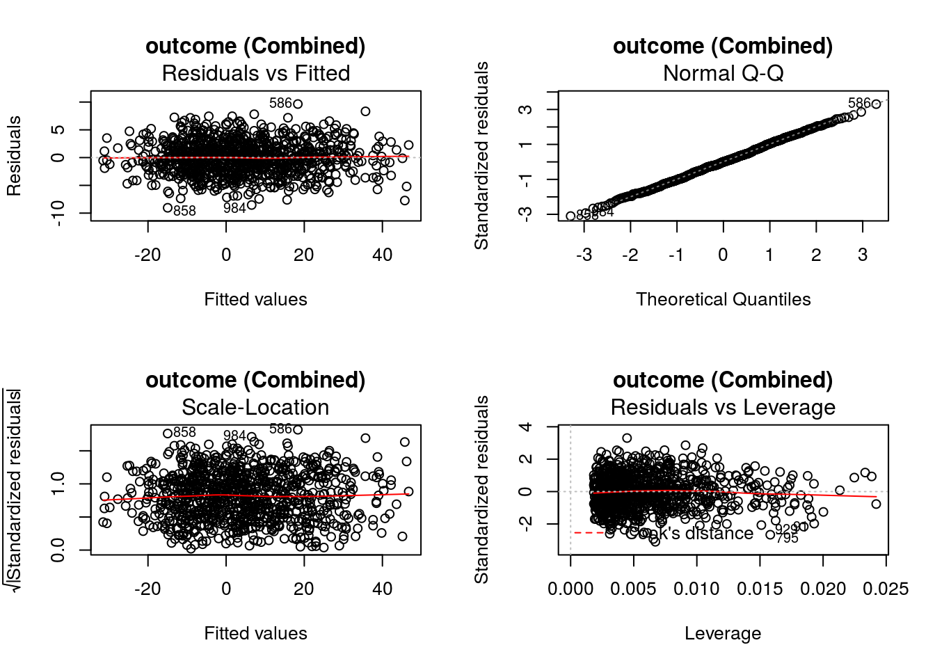
-15.6048448 -0.2034722 12.2848519 -61.0979087 0.5048157 -6.6098761 If defined by the regression methods, standard diagnostic plots can be generated using DynTxRegime::
graphics::par(mfrow = c(2,2))
DynTxRegime::plot(x = result)
The value of input variable suppress determines if the plot titles are concatenated with an identifier of the regression analysis being plotted. For example, below we plot the Residuals vs Fitted for the propensity score and outcome regressions with and without the title concatenation.
graphics::par(mfrow = c(2,2))
DynTxRegime::plot(x = result, which = 1)
DynTxRegime::plot(x = result, suppress = TRUE, which = 1)
If there are additional diagnostic tools defined for a regression method used in the analysis but not implemented in DynTxRegime, the value object returned by the regression method can be extracted using function DynTxRegime::
fitObj <- DynTxRegime::fitObject(object = result)
fitObj$propensity
Call: glm(formula = YinternalY ~ SBP0 + Ch, family = "binomial", data = data)
Coefficients:
(Intercept) SBP0 Ch
-15.94153 0.07669 0.01589
Degrees of Freedom: 999 Total (i.e. Null); 997 Residual
Null Deviance: 1378
Residual Deviance: 1162 AIC: 1168
$outcome
$outcome$Combined
Call:
lm(formula = YinternalY ~ Ch + K + A + Ch:A + K:A, data = data)
Coefficients:
(Intercept) Ch K A Ch:A K:A
-15.6048 -0.2035 12.2849 -61.0979 0.5048 -6.6099 As for DynTxRegime::
is(object = fitObj$outcome$Combined)[1] "lm" "oldClass"is(object = fitObj$propensity)[1] "glm" "lm" "oldClass"As such, these objects can be passed to any tool defined for these classes. For example, the methods available for the object returned by the propensity score regression are
utils::methods(class = is(object = fitObj$propensity)[1L]) [1] add1 anova coerce confint cooks.distance deviance drop1 effects
[9] extractAIC family formula influence initialize logLik model.frame nobs
[17] predict print residuals rstandard rstudent show slotsFromS3 summary
[25] vcov weights
see '?methods' for accessing help and source codeSo, to plot the residuals
graphics::plot(x = residuals(object = fitObj$propensity))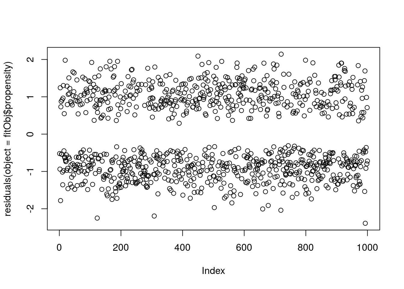
Or, to retrieve the variance-covariance matrix of the parameters
stats::vcov(object = fitObj$propensity) (Intercept) SBP0 Ch
(Intercept) 1.689875691 -8.970374e-03 -1.095841e-03
SBP0 -0.008970374 5.178554e-05 2.752417e-06
Ch -0.001095841 2.752417e-06 3.072313e-06The methods DynTxRegime::
DynTxRegime::outcome(object = result)$Combined
Call:
lm(formula = YinternalY ~ Ch + K + A + Ch:A + K:A, data = data)
Coefficients:
(Intercept) Ch K A Ch:A K:A
-15.6048 -0.2035 12.2849 -61.0979 0.5048 -6.6099 DynTxRegime::propen(object = result)
Call: glm(formula = YinternalY ~ SBP0 + Ch, family = "binomial", data = data)
Coefficients:
(Intercept) SBP0 Ch
-15.94153 0.07669 0.01589
Degrees of Freedom: 999 Total (i.e. Null); 997 Residual
Null Deviance: 1378
Residual Deviance: 1162 AIC: 1168DynTxRegime::classif(object = result)n= 1000
node), split, n, loss, yval, (yprob)
* denotes terminal node
1) root 1000 0.1401350000 1 (0.025873081 0.974126919)
2) Ch< 183.55 285 0.0166130600 0 (0.568407075 0.431592925)
4) Ch< 155.2 119 0.0017551050 0 (0.905908559 0.094091441) *
5) Ch>=155.2 166 0.0148579600 0 (0.251082865 0.748917135)
10) K>=4.25 80 0.0026340590 0 (0.552429068 0.447570932) *
11) K< 4.25 86 0.0106160000 1 (0.123987442 0.876012558)
22) W< 62.9 21 0.0012200790 0 (0.373747901 0.626252099) *
23) W>=62.9 65 0.0061481210 1 (0.083457937 0.916542063)
46) Cr< 0.75 19 0.0009908188 0 (0.315338047 0.684661953) *
47) Cr>=0.75 46 0.0033479920 1 (0.051676480 0.948323520) *
3) Ch>=183.55 715 0.0058836740 1 (0.001135832 0.998864168) *Once satisfied that the postulated models are suitable, the estimated optimal treatment and estimated value for the dataset used for the analysis can be retrieved.
Function DynTxRegime::
DynTxRegime::optTx(x = result)$optimalTx
[1] 0 0 1 1 1 1 1 0 1 1 1 1 1 0 0 1 0 0 1 1 1 1 0 1 1 1 1 1 1 1 1 1 0 1 1 1 1 1 0 1 1 1 1 0 1 1 1 0 1 1 1 1 1 1 0 0 1 1 1
[60] 1 1 1 1 1 1 1 1 1 1 1 1 1 1 1 1 0 1 0 1 1 0 1 1 1 0 1 1 1 1 1 1 1 1 1 1 1 1 1 1 1 1 1 1 0 0 0 1 1 1 1 0 1 1 0 1 1 0 1
[119] 0 1 1 1 1 1 1 0 0 0 1 1 1 1 1 0 1 1 1 1 0 1 1 1 1 1 0 1 1 1 0 1 1 1 0 1 1 0 1 1 1 1 1 1 1 0 1 1 1 1 1 0 1 0 1 0 1 1 0
[178] 1 1 1 1 1 1 1 1 0 1 1 0 1 1 1 1 1 1 1 0 1 1 1 0 0 1 0 1 1 1 1 1 0 0 0 1 1 1 0 1 1 1 1 1 1 1 1 1 1 1 1 1 1 1 1 1 0 1 1
[237] 1 1 1 0 1 0 1 0 1 1 1 1 0 1 1 1 1 1 1 1 1 1 0 0 1 0 1 1 0 1 1 0 1 0 1 1 1 0 1 1 1 1 0 1 1 1 0 1 0 1 0 1 1 1 1 1 1 0 1
[296] 1 1 1 1 1 1 1 1 1 1 1 0 1 1 0 1 1 1 1 1 0 0 1 0 1 1 1 0 1 1 0 1 1 1 1 1 1 1 1 1 1 0 1 1 1 0 1 1 1 1 1 1 1 1 1 0 1 1 1
[355] 1 0 1 1 0 1 1 1 1 1 1 1 1 0 0 1 0 0 1 0 1 1 1 1 1 1 1 0 1 0 1 1 1 1 1 0 0 1 0 1 1 0 1 1 1 1 1 1 1 1 0 1 1 0 1 1 0 1 1
[414] 1 1 1 0 1 1 1 1 1 1 1 1 1 1 1 1 1 1 1 1 1 1 1 1 1 0 1 0 1 1 0 1 1 1 1 1 0 1 0 0 0 1 1 1 1 1 1 1 1 0 1 1 1 1 1 1 1 0 1
[473] 0 1 1 1 0 1 0 1 1 1 1 0 0 0 1 1 1 1 1 1 1 1 0 0 1 1 1 1 0 0 1 0 0 1 1 0 1 1 1 0 1 1 1 1 1 1 1 0 0 1 1 1 1 1 1 1 0 1 0
[532] 0 1 1 1 0 1 1 1 0 1 0 0 1 0 1 1 1 1 0 1 1 0 0 1 0 1 1 1 1 1 1 1 1 1 1 1 1 1 0 1 1 0 1 1 0 1 1 1 0 1 0 1 1 1 1 1 0 0 1
[591] 1 1 1 1 1 1 1 0 1 0 1 1 1 1 1 1 1 0 1 0 0 1 0 1 1 1 1 1 0 0 1 1 1 1 1 0 1 1 0 0 0 1 1 0 0 1 1 1 1 1 0 1 1 1 1 1 1 1 1
[650] 1 1 1 1 1 1 0 1 1 1 1 1 1 1 1 1 0 1 1 1 1 0 1 1 1 1 1 1 1 0 0 1 0 1 1 1 1 0 0 0 0 1 1 1 1 1 0 0 1 1 1 1 1 1 1 1 1 1 1
[709] 1 1 1 1 1 1 1 0 1 0 1 1 1 1 0 1 0 1 1 1 1 1 1 1 0 1 1 0 1 0 0 1 1 0 0 1 1 1 1 1 1 1 0 1 1 0 0 1 1 1 1 1 0 0 0 1 1 1 1
[768] 0 1 1 1 1 0 1 1 1 0 1 1 1 1 1 1 1 1 1 0 1 1 1 0 0 1 0 1 1 1 1 0 1 1 1 0 1 1 1 1 1 1 0 0 1 1 0 1 0 1 1 1 1 0 1 0 1 0 0
[827] 0 1 1 1 1 0 1 1 1 1 1 1 1 1 1 1 1 0 0 1 0 1 1 1 1 1 1 1 1 1 1 1 1 1 1 1 1 0 1 0 1 1 1 1 0 1 1 0 1 0 1 0 1 1 1 0 1 1 1
[886] 1 0 0 1 1 0 1 0 1 1 1 1 1 0 1 1 1 0 1 0 1 1 1 1 1 1 0 1 1 1 1 1 1 0 1 0 1 0 0 0 0 1 0 1 1 1 1 1 1 1 1 1 1 1 0 1 1 1 1
[945] 1 0 1 1 1 1 1 1 1 1 0 1 1 1 1 0 1 0 0 1 1 1 1 1 1 1 1 1 1 1 1 1 0 1 1 0 1 1 1 1 1 0 0 1 0 1 1 0 1 0 0 0 1 1 1 1
$decisionFunc
[1] NAThe object returned is a list. Element $optimalTx corresponds to the \(\widehat{d}^{opt}_{\eta}(H_{1i}; \widehat{\eta}_{1})\); element $decisionFunc is NA as it is not defined in this context but is included for continuity across methods.
Function DynTxRegime::
DynTxRegime::estimator(x = result)[1] 13.23713Function DynTxRegime::
The first new patient has the following baseline covariates
print(x = patient1) SBP0 W K Cr Ch
1 162 72.6 4.2 0.8 209.2The recommended treatment based on the previous analysis is obtained by providing the object returned by DynTxRegime::
DynTxRegime::optTx(x = result, newdata = patient1)$optimalTx
[1] 1
$decisionFunc
[1] NATreatment A= 1 is recommended.
The second new patient has the following baseline covariates
print(x = patient2) SBP0 W K Cr Ch
1 153 68.2 4.5 0.8 178.8And the recommended treatment is obtained by calling
DynTxRegime::optTx(x = result, newdata = patient2)$optimalTx
[1] 0
$decisionFunc
[1] NATreatment A= 0 is recommended.
Outcome Weighted Learning
Here, we consider a special case of the value search estimator referred to as outcome weighted learning. Consider the estimation of an optimal restricted regime \(d^{opt}_{\eta}\) in a restricted class \(\mathcal{D}_{\eta}\) by maximizing the simple inverse probability weighted (IPW) estimator
\[ \widehat{\mathcal{V}}_{IPW} (d_{\eta}) = n^{-1} \sum_{i=1}^{n} \frac{ \mathcal{C}_{d_{\eta},i} Y_{i}}{\pi_{d_{\eta},1}(H_{1i};\eta_{1}, \widehat{\gamma}_{1})}, \]
in \(\eta=\eta_{1}\). As before, \(\mathcal{C}_{d_{\eta}}\) is the indicator of whether or not the treatment option received coincides with that recommended by \(d_{\eta}\), that is \(\mathcal{C}_{d_{\eta}} = \text{I}\{ A_{1} = d_{1}(H_{1}; \eta_{1})\}\), and \(\pi_{{d_{\eta}},1} (H_{1}; \eta_{1}, \gamma_{1})\) is the model for the propensity for receiving treatment consistent with \(d_{\eta}\) given an individual’s history, \(P(\mathcal{C}_{d_{\eta}}=1|H_{1})\).
For binary treatments coded as \(\mathcal{A}_{1} = \{0,1\}\), it can be shown that maximizing \(\mathcal{V}_{IPW}(d_{\eta})\) to obtain \(\widehat{d}^{opt}_{\eta,IPW}\) is equivalent to \[ \begin{align} \min_{\eta_{1}} n^{-1} \sum_{i=1}^{n} \left| \widehat{C}_1(H_{1i}, A_{1i}, Y_i) \right| \text{I}\Big[ \text{I}\left\{\widehat{C}_1(H_{1i}, A_{1i}, Y_i) \gt 0 \right\} \neq \text{I}\{ d_{1}(H_{1i}; \eta_{1}) = 1\}\Big], \end{align} \] where
\[ \widehat{C}_{1}(H_{1i},A_{1i},Y_{i}) = \left\{\frac{ A_{1i}}{\pi_{1}(H_{1i};\widehat{\gamma}_{1}) } - \frac{ 1 - A_{1i}}{1 - \pi_{1}(H_{1i};\widehat{\gamma}_{1}) }\right\} Y_{i} \] for the inverse probability weighted value estimator.
For binary treatment, the treatment rule \(d_{1}(h_{1}; \eta_{1})\) can be expressed as \[ d_{1}(h_{1}; \eta_{1}) = \text{I}\{ f_1(h_{1}; \eta_{1}) \gt 0\}, \] and it can be shown that maximizing \(\mathcal{V}_{IPW}(d_{\eta})\) to obtain \(\widehat{d}^{opt}_{\eta,IPW}\) is equivalent to the following minimization \[ \begin{align} \min_{\eta_{1}} n^{-1} \sum_{i=1}^{n} \left\{\frac{ A_{1i}}{\pi_{1}(H_{1i};\widehat{\gamma}_{1}) } + \frac{ 1 - A_{1i}}{1 - \pi_{1}(H_{1i};\widehat{\gamma}_{1}) }\right\}\left|Y_{i}\right| \text{I}\left[ \text{sign}(Y_{i}) (2 A_{1i} - 1) \neq \text{sign}\{f_1(h_{1}; \eta_{1})\}\right]. \\ \end{align} \]
This classifier is nonsmooth and involves a nonconvex 0-1 loss function. Such loss functions can be extremely hard to optimize, and it is common to consider a proxy (or surrogate) to the loss function, e.g., the so-called “hinge loss” function.
\[ \ell_{hinge}(x) = (1-x)^+, \hspace{0.15in} x^+ = \max(0,x). \]
By using such a surrogate, \(\ell_{s}(x)\), the minimization problem is recast as,
\[ \begin{align} \min_{\eta_{1}} n^{-1} \sum_{i=1}^{n} ~ \left\{\frac{ A_{1i}}{\pi_{1}(H_{1i};\widehat{\gamma}_{1}) } + \frac{ 1-A_{1i}}{1 - \pi_{1}(H_{1i};\widehat{\gamma}_{1}) }\right\} \left|Y_{i}\right| ~ \ell_{\scriptsize{\mbox{s}}}\{Y_{i} f_1(h_{1}; \eta_{1})(2 A_{1i} - 1)\}+ \lambda_n \| f_1\|^2, \end{align} \] where \(\| \cdot\|\) is a suitable norm for \(f_1\) and \(\lambda_n\) is a scalar tuning parameter possibly depending on \(n\). The second term in the above expression penalizes the complexity of the estimated decision function to avoid overfitting.
The minimization of the above expression in parameters \(\eta\) is called OWL, and the minimizer \(\widehat{\eta}^{opt}_{1,OWL}\) defines the estimated optimal restricted regime arising from OWL
\[ \widehat{d}^{opt}_{\eta,OWL} = \{ d_{1}(h_{1}; \widehat{\eta}^{opt}_{1,OWL}) \} = \text{I}\{ f_1(h_{1}; \widehat{\eta}^{opt}_{1,OWL}) \gt 0\}. \]
The development of the estimator here differs from that of the book. The original manuscript assumed that the outcome is positive, which is maintained in the discussion of the estimator in the book. However, this is not a requirment, and the implementation of DynTxRegime does not make this assumption.
A general implementation of the OWL estimator is provided in
utils::str(object = DynTxRegime::owl)function (..., moPropen, data, reward, txName, regime, response, lambdas = 2, cvFolds = 0L, kernel = "linear", kparam = NULL,
surrogate = "hinge", verbose = 2L) We briefly describe the input arguments for DynTxRegime::
| Input Argument | Description |
|---|---|
| \(\dots\) | Used primarily to require named input. However, inputs for the optimization methods can be sent through the ellipsis. |
| moPropen | A “modelObj” object. The modeling object for the propensity score regression step. |
| data | A “data.frame” object. The covariate history and the treatment received. |
| reward | A “numeric” vector. The outcome of interest, where larger values are better. This input is equivalent to response. |
| txName | A “character” object. The column header of data corresponding to the treatment variable. |
| regime | A “formula” object or a character vector. The covariates to be included in classification. |
| response | A “numeric” vector. The outcome of interest, where larger values are better. |
| lambdas | A “numeric” object or a “numeric” vector. One or more penalty tuning parameters. |
| cvFolds | An “integer” object. The number of cross-validation folds. |
| kernel | A “character” object. The kernel of the decision function. Must be one of {linear, poly, radial} |
| kparam | A “numeric” object, a “numeric” “vector”, or NULL. The kernel parameter when required. |
| surrogate | A “character” object. The surrogate 0-1 loss function. Must be one of {logit, exp, hinge, sqhinge, huber} |
| verbose | A “numeric” object. If \(\ge 2\), all progress information is printed to screen. If =1, some progress information is printed to screen. If =0 no information is printed to screen. |
Though the OWL method has was developed in the original manuscript in the notation of \(\mathcal{A} \in \{-1,1\}\) and \(Y \gt 0\), these are not a requirment of the implementation in DynTxRegime. It is only required that treatment be binary and coded as either integer or factor and that larger values of \(Y\) are preferred.
The value object returned by DynTxRegime::
| Slot Name | Description |
|---|---|
| @analysis@txInfo | The treatment information. |
| @analysis@propen | The propensity regression analysis. |
| @analysis@outcome | NA; outcome regression is not a component of this method. |
| @analysis@cvInfo | The cross validation results. |
| @analysis@optim | The final optimization results. |
| @analysis@call | The unevaluated function call. |
| @analysis@optimal | The estimated value, decision function, and optimal treatment for the training data. |
There are several methods available for objects of this class that assist with model diagnostics, the exploration of training set results, and the estimation of optimal treatments for future patients. We explore these methods under the Methods tab.
We continue to consider the propensity score models introduced in Chapter 2, which represent a range of model (mis)specification. For brevity, we discuss the function call to DynTxRegime::
Input moPropen is a modeling object for the propensity score regression. To illustrate, we will use the true propensity score model
\[ \pi^{3}_{1}(h_{1};\gamma_{1}) = \frac{\exp(\gamma_{10} + \gamma_{11}~\text{SBP0} + \gamma_{12}~\text{Ch})}{1+\exp(\gamma_{10} + \gamma_{11}~\text{SBP0}+ \gamma_{12}~\text{Ch})}, \] which is defined as a modeling object as follows
p3 <- modelObj::buildModelObj(model = ~ SBP0 + Ch,
solver.method = 'glm',
solver.args = list(family='binomial'),
predict.method = 'predict.glm',
predict.args = list(type='response'))As for all methods discussed in this chapter: the “data.frame” containing the baseline covariates and treatment received is data set dataSBP, the treatment is contained in column $A of dataSBP, and the outcome of interest is the change in systolic blood pressure measured six months after treatment, \(y = \text{SBP0} - \text{SBP6}\), which is already defined in our R environment.
The outcome of interest can be provided through either input response or input reward. This “option” for how the outcome is provided is not the standard styling of inputs for
The decision function \(f_{1}(H_{1};\eta_{1})\) is defined using a kernel function. Specifically,
\[ f_{1}(H_1;\eta_{1}) = \sum_{i=1}^{n} \eta_{i} A_{1i} k(H_1,H_{1i}) + \eta_0 \]
where \(k(X,X_{i})\) is a continuous, symmetric, and positive definite kernel function. At this time, three kernel functions are implemented in DynTxRegime:
\[ \begin{array}{lrl} \textrm{linear} & k(x,y) = &x^{\intercal} y; \\ \textrm{polynomial} & k(x,y) = &(x^{\intercal} y + c)^{\color{red}d}; ~ \textrm{and}\\ \textrm{radial basis function} & k(x,y) = &\exp(-||x-y||^2/(2 {\color{red}\sigma}^2)). \end{array} \]
Notation shown in \(\color{red}{red}\) indicates the kernel parameter that must be provided through input kparam. Note that the linear kernel does not have a kernel parameter.
For this illustration, we specify a linear kernel and will include baseline covariates Ch and K in the kernel. Thus,
kernel <- 'linear'
regime <- ~ Ch + K
kparam <- NULLTo illustrate the cross-validation capability of the implementation, we will consider five tuning parameters and use 10-fold cross-validation to determine the optimal.
lambdas <- 10^{seq(from = -4, to = 0, by = 1)}
cvFolds <- 10LCurrently, five surrogates for the 0-1 loss function are available.
\[ \begin{array}{crlc} \textrm{hinge} & \phi(t) = & \max(0, 1-t) & \textrm{"hinge"}\\ \textrm{square-hinge} & \phi(t) = & \{\max(0, 1-t)\}^2 & \textrm{"sqhinge"}\\ \textrm{logistic} & \phi(t) = & \log(1 + e^{-t}) & \textrm{"logit"}\\ \textrm{exponential} & \phi(t) = & e^{-t} & \textrm{"exp"}\\ \textrm{huberized hinge} & \phi(t) = &\left\{\begin{array}{cc} 0 & t \gt 1 \\ \frac{1}{4}(1-t)^2 & -1 \lt t \le 1 \\ -t & t \le -1 \end{array}\right. & \textrm{"huber"} \end{array} \]
We will use the hinge surrogate function in this illustration, which was that chosen in the original manuscript.
When the hinge surrogate is used, R function kernlab::
Circumstances under which this input would be utilized are not represented by the data sets generated for illustration in this chapter.
The ellipsis is used in the function call primarily to require named inputs. However, for methods that have hard-coded optimization routines, the ellipsis can be used to modify default settings of those moethods. Here, by selecting the hinge surrogate, kernlab::
The optimal treatment regime is estimated as follows.
OWL3 <- DynTxRegime::owl(moPropen = p3,
data = dataSBP,
reward = y,
txName = 'A',
regime = regime,
lambdas = lambdas,
cvFolds = cvFolds,
kernel = kernel,
kparam = kparam,
surrogate = 'hinge',
verbose = 1L,
sigf = 4L)Outcome Weighted Learning
Propensity for treatment regression.
Regression analysis for moPropen:
Call: glm(formula = YinternalY ~ SBP0 + Ch, family = "binomial", data = data)
Coefficients:
(Intercept) SBP0 Ch
-15.94153 0.07669 0.01589
Degrees of Freedom: 999 Total (i.e. Null); 997 Residual
Null Deviance: 1378
Residual Deviance: 1162 AIC: 1168
Outcome regression.
No outcome regression performed.
Cross-validation for lambda = 1e-04
Fold 1 of 4
value: 12.06527
Fold 2 of 4
value: 14.0078
Fold 3 of 4
value: 13.69267
Fold 4 of 4
value: 12.02644
Average value over successful folds: 12.94804
Cross-validation for lambda = 0.001
Fold 1 of 4
value: 12.10171
Fold 2 of 4
value: 14.0078
Fold 3 of 4
value: 13.69616
Fold 4 of 4
value: 12.03503
Average value over successful folds: 12.96017
Cross-validation for lambda = 0.01
Fold 1 of 4
value: 12.21396
Fold 2 of 4
value: 14.04033
Fold 3 of 4
value: 13.7196
Fold 4 of 4
value: 12.13795
Average value over successful folds: 13.02796
Cross-validation for lambda = 0.1
Fold 1 of 4
value: 12.06122
Fold 2 of 4
value: 14.18247
Fold 3 of 4
value: 13.75772
Fold 4 of 4
value: 12.22394
Average value over successful folds: 13.05634
Cross-validation for lambda = 1
Fold 1 of 4
value: 12.06584
Fold 2 of 4
value: 14.23879
Fold 3 of 4
value: 13.70727
Fold 4 of 4
value: 12.22394
Average value over successful folds: 13.05896
Selected parameter: lambda = 1
Final optimization step.
Optimization Results
Kernel
kernel = linear
kernel model = ~Ch + K - 1
lambda= 1
Surrogate: HingeSurrogate
$par
[1] -5.75506934 0.08032119 -1.98124425
$convergence
[1] 0
$primal
[1] 6.873556e+00 4.657247e+00 5.106701e-06 2.981781e-06 9.246049e-07 9.597590e-07 6.871795e-06 1.043197e-05
[9] 1.501977e-06 2.992898e-05 5.035653e-06 1.619768e-06 1.906394e-06 3.905800e-06 1.906762e-06 6.154095e-07
[17] 8.819572e-05 2.451868e+00 4.337689e-06 6.383995e+00 2.903864e-05 1.892639e-05 3.980216e-04 1.206569e-06
[25] 1.950819e-06 1.282073e-06 3.911418e-05 2.906042e+00 1.234596e+01 7.353848e-06 5.151198e-05 1.623686e-06
[33] 3.648197e-05 5.588648e-06 1.319061e-06 3.351841e-06 7.426202e-07 7.749054e-06 8.932081e-06 3.898903e+00
[41] 9.042022e-07 1.431585e-06 1.234014e+01 8.600996e-06 1.674982e-06 5.640163e-06 1.501046e-05 7.676570e+00
[49] 3.775985e-06 2.304210e-06 8.459197e-07 2.386426e-06 8.156490e-06 1.542500e-06 2.419347e+00 2.956433e+00
[57] 2.007562e+01 2.260438e-06 3.030299e-06 5.852073e-06 9.553212e-07 6.738840e-06 1.927378e-06 1.213955e+00
[65] 1.000203e-05 1.470451e-06 8.109897e-06 8.421970e-07 2.553754e-05 2.431442e-06 8.863231e-07 9.507030e-05
[73] 4.500071e+00 1.136945e-06 8.680452e-06 3.207135e+00 1.818313e-06 1.515013e-05 1.326749e-05 4.140881e-06
[81] 2.142818e-06 1.720645e-06 2.539102e-06 2.001614e-06 2.401843e+00 9.539406e-07 2.073969e-06 2.954198e-06
[89] 1.774194e-06 1.387464e-05 1.463331e-06 1.854768e-05 1.347585e-06 2.063177e-06 4.403948e-06 1.189050e-05
[97] 1.197826e-05 8.775103e+00 2.738453e-06 4.615364e-06 1.611471e-06 7.657638e+00 6.853290e-06 8.405002e+00
[105] 1.899728e+01 7.849689e+00 7.997949e-06 2.077774e-06 1.338634e-06 9.651069e-07 2.429046e+00 2.150596e-06
[113] 1.358498e-07 8.106668e-04 4.878514e-06 6.544108e-06 1.085614e-06 1.813783e-06 6.525793e-07 1.532782e-06
[121] 3.206767e-06 4.043113e-06 2.619555e-06 1.108182e-06 7.551297e-06 3.737253e+00 9.824145e+00 2.029590e-06
[129] 6.660948e-06 1.860035e-06 2.900422e-05 1.308718e-06 9.164774e-06 1.381377e-06 7.300218e-07 1.454820e-06
[137] 7.530804e-07 1.598348e-06 2.066005e-06 2.680144e+01 1.827257e-06 9.183238e-07 3.253138e-06 1.644897e-06
[145] 6.947895e-06 3.992548e-06 1.166745e-04 4.420271e-06 1.611371e-05 1.002982e-05 2.304803e-06 2.036393e+01
[153] 1.159259e+00 2.431749e-06 9.215265e-07 1.029387e-04 1.546214e-06 1.415615e-05 2.811181e-06 5.570449e-07
[161] 1.171754e-06 2.216872e-06 3.222194e-06 2.719045e-05 7.732508e-07 6.911084e-07 1.608750e-05 5.328921e-06
[169] 8.858609e+00 1.159535e+01 2.421942e-06 1.551132e-05 1.568572e-06 2.530809e+00 1.016018e-05 1.039737e-05
[177] 1.682590e+01 4.497012e-06 1.619807e-05 1.603679e-06 1.840136e-06 1.644458e-06 1.771287e-06 3.618823e+00
[185] 5.702407e-08 6.330776e-06 1.781478e-06 1.079411e-05 7.323136e-06 1.319221e-06 2.966583e-06 9.559159e-06
[193] 3.273696e-06 1.769214e-05 1.490826e-05 4.362198e-05 7.393955e+00 2.276967e-06 1.008754e+01 1.921752e-06
[201] 1.247344e+01 8.705479e+00 1.252194e-06 6.049455e-07 9.919583e-06 3.751771e-06 8.491942e+00 7.532467e-06
[209] 2.810601e-06 2.017192e-05 1.003291e-05 1.216382e-06 4.281872e-06 3.883019e+00 1.600168e-06 3.279983e+00
[217] 2.690857e-06 5.929992e-06 6.660891e-06 7.221689e-07 1.704446e-06 1.890098e-06 7.475737e-06 2.065270e-06
[225] 2.606816e-06 3.243437e-06 1.168296e-06 6.523021e-07 1.833274e-06 1.884449e-05 7.767792e-06 5.572505e-06
[233] 1.750530e-05 2.380561e-06 1.380626e+01 4.500989e+00 6.960950e+00 1.941265e-06 2.055829e-05 2.043687e-06
[241] 1.422132e-05 1.551424e-06 1.713728e-05 7.901147e-07 1.213917e-06 2.186248e-06 1.508107e-05 8.454871e-07
[249] 9.508142e-06 8.481545e-07 9.401070e-06 1.857933e-06 1.892970e-06 9.781230e-06 1.628963e-06 1.462891e+00
[257] 4.336339e-06 6.957182e-07 7.031923e-06 1.311999e-05 7.981694e+00 3.512308e-06 3.494660e-06 1.382985e-06
[265] 2.126885e-05 1.296140e-05 7.292223e+00 5.064854e-07 3.372556e+00 1.836356e+00 2.445547e-05 2.579417e-05
[273] 1.769489e-06 1.105611e-05 1.420603e-05 1.972505e-05 1.514624e-06 1.118285e-06 1.331511e-04 2.164123e-06
[281] 1.463238e+00 1.141021e-06 2.057116e-05 4.846372e-06 2.522974e-04 2.796419e-06 8.801523e-05 1.503603e-06
[289] 1.277991e-06 1.113753e+01 2.861923e+00 2.279513e-06 1.165970e-05 7.772586e-07 1.358655e-06 8.369730e-07
[297] 1.575290e-05 4.289476e-06 1.595124e-05 1.706543e-06 1.396286e-06 4.072491e-07 5.432571e-05 1.536904e-06
[305] 1.008171e-05 4.850381e-06 4.838665e-04 3.788624e-06 1.146769e-05 1.860858e-06 2.623765e-06 1.149784e-06
[313] 6.713227e-06 2.013453e-06 3.674315e+00 2.259658e-06 1.150590e-04 3.446340e-06 1.491140e-05 2.350382e-06
[321] 6.105583e-06 1.578098e-06 1.877754e-05 1.043511e-06 2.285141e-05 6.073511e-06 6.894056e-06 2.139373e-06
[329] 1.532434e-06 1.233880e-05 1.608236e-06 1.739949e-06 7.367665e-06 1.120076e-06 1.084794e-05 2.790922e-05
[337] 6.723467e+00 2.898775e-06 1.187144e-05 5.278012e+00 1.489167e+00 9.360910e-07 1.210606e-06 1.358961e+00
[345] 2.813112e-06 3.107577e-05 1.154593e+01 1.834749e+01 5.720728e-07 1.290534e-06 6.505052e-06 4.166213e-06
[353] 8.373605e-07 4.261563e+00 1.267094e-05 8.732648e-06 1.086549e-06 2.104652e-06 1.433705e+01 1.674457e-06
[361] 3.306366e+00 2.066047e-06 1.407514e-06 1.168992e-06 7.957716e-07 8.783710e-07 8.046564e-06 6.590045e-06
[369] 5.998224e+00 1.373389e-06 5.363786e-05 1.158095e+01 5.170785e-07 5.759540e+00 1.703521e-06 8.049722e-07
[377] 1.621297e-06 2.295575e-06 4.379179e-06 3.043769e-06 1.602467e-06 3.112470e-05 5.254528e-06 1.172145e-05
[385] 1.653775e-06 7.811287e-06 1.471168e+01 1.502355e-06 4.487657e-07 8.521291e-07 3.558868e-07 2.205380e-05
[393] 8.388396e-07 1.691319e-06 5.592519e-06 3.080577e-05 1.121367e-04 1.101031e-06 1.129947e+00 2.010680e-06
[401] 2.158283e-06 1.482254e-05 3.478671e-07 1.405019e-06 3.163184e+00 1.328981e-06 1.805157e-06 1.712344e-05
[409] 3.687520e+01 1.488534e-06 1.240279e+01 7.551918e-07 3.235619e-06 3.796425e+00 2.305315e-06 1.381701e-06
[417] 7.513180e-07 1.379247e-06 1.425334e-06 2.534429e-06 1.884643e-05 8.299046e+00 8.062651e-06 1.177986e+00
[425] 5.943294e-06 2.158562e-06 1.811220e-06 5.756718e-05 1.745599e-05 1.067576e-05 2.343941e+01 4.261483e-06
[433] 9.873341e-07 8.135991e-06 8.991383e-06 3.246291e-06 1.591950e-06 2.182223e-05 1.891456e-05 1.001720e-05
[441] 1.628779e-05 2.738355e-05 3.283522e-06 4.576291e-06 5.014164e+00 5.278469e-06 5.621029e-06 7.660989e-07
[449] 2.987437e-06 8.889956e+00 5.499893e+00 2.717602e-06 1.478566e-05 7.826204e+00 1.574141e-06 3.310646e+00
[457] 1.600472e-06 2.587352e-06 1.934184e-06 2.624585e-06 4.864710e+00 1.921724e-05 3.356954e-06 1.743194e-06
[465] 1.158325e-05 4.217629e-06 2.820583e-05 1.195941e-06 1.783254e-06 2.205221e-06 3.508968e+00 4.070518e-05
[473] 2.184504e+00 1.650395e-06 1.819749e-05 2.072180e-06 9.309101e-07 2.975507e-06 1.613539e+01 8.474677e-06
[481] 1.728521e-06 3.384396e-05 1.257328e-05 6.173236e+00 1.254685e+01 6.911822e-07 5.940012e-06 1.554367e-05
[489] 1.329055e-06 2.373544e-06 3.553258e-06 2.195423e-06 5.066288e+00 3.040800e-06 3.788305e-06 1.913462e-06
[497] 1.152809e-06 1.018940e-05 1.107177e-06 1.756721e-05 2.383121e-05 5.664392e+00 3.127241e-06 1.079089e-06
[505] 5.155335e+00 9.534125e-07 6.597232e-06 1.645748e-06 7.749531e-06 3.137326e-06 1.799872e-06 1.180672e-06
[513] 5.774124e-07 2.704326e-05 1.496779e-06 2.421307e+01 1.458130e-06 1.223729e-06 4.788583e+00 2.641538e+00
[521] 1.441938e+01 1.557087e-06 1.630147e-06 6.962753e-06 1.700056e-06 1.121387e+01 2.700984e-05 8.918602e-07
[529] 1.266799e-05 1.873829e-06 5.344927e-06 4.597767e+00 2.252153e-06 1.652426e-05 3.379010e-06 2.598736e+01
[537] 4.459612e+00 1.654820e-05 3.532114e-06 1.304161e+01 2.994507e-06 4.434053e+00 1.009581e-06 9.198604e-06
[545] 4.794401e+00 2.520048e+01 1.919049e-06 1.339184e-06 4.381266e-06 3.337904e+00 2.215701e-06 6.745580e-06
[553] 1.971723e+01 8.061595e-06 2.957697e-06 1.617830e-05 6.131109e-07 2.233828e+00 1.576413e-06 2.521830e-06
[561] 2.069663e-06 6.523471e-07 1.308491e-06 1.126095e-06 5.802564e-06 2.222031e-06 3.479313e-06 5.707889e-05
[569] 1.227204e-06 1.174927e-05 3.308685e-05 2.895823e+01 3.599961e+00 1.025662e+01 9.444211e-07 3.744196e-05
[577] 4.301738e-05 8.598421e-06 3.901502e-06 2.991384e-06 4.280316e-04 8.423774e-06 1.313119e-06 2.183209e-06
[585] 2.670451e-06 2.233576e-06 1.611080e-06 2.585237e+01 1.112346e-05 1.087595e-04 3.228845e-06 6.127165e+00
[593] 2.644160e-06 1.611416e+00 1.860679e-06 8.488063e-05 1.613582e-06 4.964472e+00 7.269218e-06 7.117589e+00
[601] 6.351525e-06 9.688279e-07 2.617362e-06 2.202255e-05 1.515840e-06 1.785023e-06 9.573140e-06 6.113995e+00
[609] 1.583987e-06 6.647305e-06 3.422223e-06 6.667197e+00 1.472788e-05 2.544582e-06 8.301199e-07 4.369024e-05
[617] 1.445019e+01 1.654504e-06 9.703840e-06 9.624543e-06 8.148030e-07 1.984633e-05 6.814134e-06 1.098029e-06
[625] 2.119843e-06 9.979006e-06 1.623211e-06 1.415493e+01 3.182965e+01 3.720145e-06 8.409961e-07 4.617071e-06
[633] 1.767473e-06 3.478914e-06 2.707678e-05 1.443430e-06 1.955787e-06 2.452708e-06 3.743277e+00 2.436503e-05
[641] 9.103229e-06 2.554043e-06 1.413420e+01 7.742375e+00 1.553677e-06 3.148470e-05 1.185113e-06 2.454023e-05
[649] 7.973501e-06 5.968659e-06 3.648974e-06 6.365416e-05 1.050821e-06 1.612589e-06 1.158893e-06 2.393666e-05
[657] 9.795645e+00 2.524035e-06 7.675789e-06 3.483122e-06 1.234079e-05 1.376970e+00 6.542591e-06 6.923186e-06
[665] 3.231858e-06 1.123598e-05 2.104683e+01 1.947552e-06 2.680976e-06 2.963584e-06 6.717651e-06 1.024319e-06
[673] 1.763290e-06 6.911439e-06 5.231229e-06 5.809598e-07 1.901524e-06 3.300890e-06 1.131215e-05 1.383755e-05
[681] 1.939463e-05 3.532049e-05 1.132365e-06 1.378871e-06 1.433670e-05 5.260864e+00 8.853876e-06 6.763967e+00
[689] 7.047821e-06 1.437290e+00 7.654391e-06 5.692082e-06 2.175716e-06 1.852276e-06 2.208420e-06 4.632655e-06
[697] 4.586765e+00 1.275404e-06 1.025153e-05 3.887399e+00 5.861782e-07 2.154206e-05 1.417178e-06 1.241876e-05
[705] 1.577730e-06 1.100272e-05 1.980957e-06 2.109610e-06 1.193494e-05 1.087814e-06 5.028777e-06 1.127596e-05
[713] 1.237230e-06 2.648001e-06 9.254586e-06 3.419552e-06 1.151552e-06 6.484018e-07 3.230554e-06 2.944221e-05
[721] 5.975583e-06 5.082122e-06 2.994790e-06 4.425161e+00 1.638408e-05 1.391487e+01 2.044671e-05 5.123160e-05
[729] 1.904957e-06 5.436360e+00 1.515506e+01 5.040746e-06 5.174684e-06 1.446797e-05 3.656896e+00 1.791798e+00
[737] 4.471007e+00 9.353591e-06 2.606844e+00 3.418910e-05 8.050281e-06 6.521531e-07 7.238356e-07 6.158874e-06
[745] 2.818332e-05 2.694629e-05 6.774904e-06 4.291080e-06 5.902674e-06 5.304666e+00 1.409479e-04 1.198330e-06
[753] 5.955574e-06 3.429157e-05 2.185246e-06 2.746278e-06 2.091255e-06 1.090214e-06 1.769329e-06 1.803090e-07
[761] 1.277058e-05 1.185558e-05 8.768219e-06 2.133831e+01 1.140797e-06 2.226362e-06 1.486790e-06 1.789481e-05
[769] 1.243324e-05 1.633233e-06 6.158378e-06 1.385853e-06 1.996930e+00 3.408643e-06 1.559624e-05 3.084488e-06
[777] 1.074480e+00 1.218312e-06 1.508525e-06 3.426928e-06 1.410408e+00 2.328327e-06 9.925391e-06 3.776070e-06
[785] 1.151594e-05 4.032313e+00 8.307235e-07 5.487505e+00 1.356406e-06 9.755810e-05 1.731043e-05 7.826254e-06
[793] 3.439329e-06 2.754777e+00 -2.147536e-07 1.374018e-06 1.336902e-06 1.186350e-05 2.616627e-05 4.477412e-06
[801] 1.803859e-06 1.567605e-05 4.322946e+00 1.569052e-06 3.179378e-06 9.982684e-04 4.176840e-06 1.683723e-06
[809] 1.973859e-06 6.339733e-06 1.400472e-05 3.378011e-06 3.413158e-06 1.653048e-06 4.498620e-06 8.142813e-06
[817] 1.475863e-05 2.876150e-06 5.430329e-06 1.305331e-06 3.327283e-05 6.223660e-06 9.309852e-06 1.505560e-05
[825] 1.204639e+00 7.823386e-06 2.193665e+00 8.858419e-07 1.093855e-05 1.031407e-06 1.242439e-05 3.961051e+00
[833] 1.824872e+00 4.564802e-06 6.757754e-06 1.892671e-06 1.114680e-06 4.125942e-06 1.514998e-05 6.508761e+00
[841] 1.887789e-06 1.879186e-05 1.679798e+01 9.839869e-06 1.074342e+01 1.555275e-06 5.651741e-06 4.063173e-06
[849] 8.139668e+00 2.019085e-06 8.812425e-06 3.958938e+00 7.837036e-07 4.327953e-06 5.811018e-06 1.350807e-06
[857] 1.995994e-06 1.215574e-06 1.287648e-05 1.474086e-06 1.295887e-06 5.552727e+00 2.299294e-05 2.473201e-05
[865] 8.449547e-06 3.123635e-05 1.198202e-05 6.557389e+00 1.350342e+00 7.704020e-05 2.922826e+00 1.408297e+01
[873] -3.622712e-07 7.508582e+00 1.281904e-06 4.823106e+00 2.660025e-06 1.129524e+00 6.819210e+00 1.583382e-06
[881] 4.756847e-05 2.468830e-06 2.380756e-06 4.199990e-05 5.472652e-06 4.868512e-06 4.509428e-07 3.394535e+00
[889] 8.951630e-07 1.186789e-06 9.716664e-05 1.289149e-05 3.293812e+00 1.096852e-06 1.034599e-05 1.333611e-06
[897] 2.052456e-06 1.345108e-06 6.434753e-07 3.327813e-06 3.929979e-05 1.279050e-06 7.399274e+00 2.626913e-06
[905] 3.941479e-05 4.295140e-06 1.829434e+01 8.637439e-06 5.231672e-07 1.591133e-06 1.552407e-06 3.423760e-05
[913] 2.230294e-06 2.243877e-06 3.138515e-05 6.098471e+00 5.318412e-05 1.035834e-06 8.833080e+00 2.389325e-05
[921] 8.683605e-05 1.595377e-06 1.020842e+01 7.663074e-06 2.270173e-06 4.693839e+00 1.677774e-06 1.041709e-05
[929] 1.221386e-06 4.174673e+00 8.345359e-07 2.866877e-06 3.677257e-06 4.956129e-06 4.029673e-06 6.558626e-06
[937] 3.113338e-06 2.483100e-05 9.995025e-06 5.250474e+00 1.220440e-06 8.001874e+00 1.301669e-06 5.845981e+00
[945] 1.039287e-06 8.307058e-05 3.109214e-04 1.237236e-05 4.352267e-06 1.862792e-06 7.262535e-07 1.504184e-06
[953] 2.203199e-05 9.336520e-06 6.385393e-06 1.336054e-06 1.302054e-06 1.902567e-06 5.330166e-05 2.427296e-05
[961] 9.983060e-06 2.810382e+00 2.222910e-05 9.382884e+00 8.004816e-06 1.856674e-06 2.109004e-06 1.996171e-06
[969] 3.677416e+00 4.226833e-05 4.774700e-06 5.015288e+00 7.693848e-07 6.829492e-06 5.723514e-06 2.664118e-06
[977] 2.009907e-06 4.764882e-06 8.849059e-07 5.427677e-06 5.994648e+00 9.281181e-07 2.241497e-06 4.439139e+00
[985] 1.217583e-06 5.870097e-06 1.112359e+00 8.314747e-06 4.573914e-06 1.902597e-06 1.238069e-06 1.241940e-06
[993] 4.905891e-06 1.017235e-05 5.928876e-07 9.778536e-06 9.263434e-06 2.378388e-05 7.806794e-06 9.495827e-06
$dual
[1] 5.755069
$how
[1] "converged"
Recommended Treatments:
0 1
229 771
Estimated value: 13.07951 The verbose output generated can be extensive due in part to the cross-validation selection. Selecting verbose = 1, limits the printing of the intermediate optimization steps performed during the cross-validation. Notice the following:
- The first lines of the verbose output indicates that the selected value estimator is the outcome weighted learning estimator.
- The information provided for the propensity score regression is not defined within DynTxRegime::
owl() , but is specified by the statistical method selected to obtain parameter estimates; in this example it is defined by stats::glm() .
Users should verify that the model was correctly interpreted by the software and that there are no warnings or messages reported by the regression method. - A statement indicates that no outcome regression was performed; this is expected for the OWL method.
- The intermediate results of the cross-validation procedure follow the regression model analyses. In our example, only the value for each fold is shown; the optimization results for each fold are suppressed because verbose = 1. After all cross-validation steps, the selected \(\lambda\) is displayed. The selected \(\lambda\) is the tuning parameter that yields the largest average value across folds. If more than one \(\lambda\) meets this criterion, the smallest of them is selected.
- Finally, a tabled summary of the recommended treatments and the estimated value for the training data are shown. The sum of the elements of the table should be the number of individuals in the training data. If it is not, the data set is likely not complete; method implementation in DynTxRegime require complete data sets.
The first step of the post-analysis should always be model diagnostics. DynTxRegime comes with several tools to assist in this task. However, we have explored the outcome regression models previously and will skip that step here. Available model diagnostic tools are described under the Methods tab.
The estimated parameters of the optimal treatment regime can be retrieved using DynTxRegime::
DynTxRegime::regimeCoef(object = OWL3)[1] -5.75506934 0.08032119 -1.98124425Thus the estimated optimal treatment decision function is
\[ f_{1}(H_{1};\widehat{\eta}_{1}) = - 5.76 + 0.08 \textrm{Ch}- 1.98 \textrm{K} = - 0.95 + 0.01 \textrm{Ch}- 0.33 \textrm{K}. \]
There are several methods available for the returned object that assist with model diagnostics, the exploration of training set results, and the estimation of optimal treatments for future patients. A complete description of these methods can be found under the Methods tab.
In the table below, we show the estimated value obtained using the OWL estimator under each of the propensity score models considered.
| (mmHg) | \(\pi^{1}_{1}(h_{1};\gamma_{1})\) | \(\pi^{2}_{1}(h_{1};\gamma_{1})\) | \(\pi^{3}_{1}(h_{1};\gamma_{1})\) |
| \(\widehat{\mathcal{V}}_{OWL}(d^{opt})\) | 16.95 | 13.12 | 13.04 |
| (\(n_{\widehat{d}=0},n_{\widehat{d}=1}\)) | \(\pi^{1}_{1}(h_{1};\gamma_{1})\) | \(\pi^{2}_{1}(h_{1};\gamma_{1})\) | \(\pi^{3}_{1}(h_{1};\gamma_{1})\) |
| OWL | (229, 771) | (240, 760) | (240, 760) |
We illustrate the methods available for objects of class “OWL” by considering the following analysis:
p3 <- modelObj::buildModelObj(model = ~ SBP0 + Ch,
solver.method = 'glm',
solver.args = list(family='binomial'),
predict.method = 'predict.glm',
predict.args = list(type='response'))result <- DynTxRegime::owl(moPropen = p3,
data = dataSBP,
reward = y,
txName = 'A',
regime = ~Ch + K,
lambdas = 10.0^{seq(from = -4, to = 0, by = 1)},
cvFolds = 10L,
kernel = 'linear',
kparam = NULL,
surrogate = 'hinge',
verbose = 0L,
sigf = 4L)| Function | Description |
|---|---|
| Call(name, …) | Retrieve the unevaluated call to the statistical method. |
| coef(object, …) | Retrieve estimated parameters of postulated propensity model(s). |
| cvInfo(object, …) | Retrieve the cross-validation values. |
| DTRstep(object) | Print description of method used to estimate the treatment regime and value. |
| estimator(x, …) | Retrieve the estimated value of the estimated optimal treatment regime for the training data set. |
| fitObject(object, …) | Retrieve the regression analysis object(s) without the modelObj framework. |
| optimObj(object, …) | Retrieve the final optimization results. |
| optTx(x, …) | Retrieve the estimated optimal treatment regime and decision functions for the training data. |
| optTx(x, newdata, …) | Predict the optimal treatment regime for new patient(s). |
| plot(x, suppress = FALSE, …) | Generate diagnostic plots for the regression object (input suppress = TRUE suppresses title changes indicating regression step.). |
| print(x, …) | Print main results. |
| propen(object, …) | Retrieve the regression analysis for the propensity score regression step |
| regimeCoef(object, …) | Retrieve the estimated parameters of the optimal restricted treatment regime. |
| show(object) | Show main results. |
| summary(object, …) | Retrieve summary information from regression analyses. |
The unevaluated call to the statistical method can be retrieved as follows
DynTxRegime::Call(name = result)DynTxRegime::owl(sigf = 4L, moPropen = p3, data = dataSBP, reward = y,
txName = "A", regime = ~Ch + K, lambdas = 10^{
seq(from = -4, to = 0, by = 1)
}, cvFolds = 10L, kernel = "linear", kparam = NULL, surrogate = "hinge",
verbose = 0L)The returned object can be used to re-call the analysis with modified inputs.
For example, to complete the analysis with a different surrogate for the 0-1 loss function requires only the following code.
surrogate <- 'sqhinge'
result_exp <- eval(expr = DynTxRegime::Call(name = result))This function provides a reminder of the analysis used to obtain the object.
DynTxRegime::DTRstep(object = result)Outcome Weighted LearningThe
DynTxRegime::summary(object = result)$propensity
Call:
glm(formula = YinternalY ~ SBP0 + Ch, family = "binomial", data = data)
Deviance Residuals:
Min 1Q Median 3Q Max
-2.3891 -0.9502 -0.4940 0.9939 2.1427
Coefficients:
Estimate Std. Error z value Pr(>|z|)
(Intercept) -15.941527 1.299952 -12.263 <2e-16 ***
SBP0 0.076687 0.007196 10.657 <2e-16 ***
Ch 0.015892 0.001753 9.066 <2e-16 ***
---
Signif. codes: 0 '***' 0.001 '**' 0.01 '*' 0.05 '.' 0.1 ' ' 1
(Dispersion parameter for binomial family taken to be 1)
Null deviance: 1377.8 on 999 degrees of freedom
Residual deviance: 1161.6 on 997 degrees of freedom
AIC: 1167.6
Number of Fisher Scoring iterations: 3
$outcome
[1] NA
$cvInfo
0 0.001 0.01 0.1 1
12.98996 12.98213 13.02685 13.07222 13.06448
$optim
$optim$par
[1] -5.95195289 0.07819043 -1.84585674
$optim$convergence
[1] 0
$optim$primal
[1] 6.873585e-01 4.657276e-01 2.098597e-07 2.090176e-08 3.548702e-08 2.597633e-08 2.233927e-07 3.736546e-07
[9] 6.508203e-08 9.103840e-07 1.585779e-07 5.065093e-08 5.329653e-08 1.331259e-07 9.419309e-08 7.150605e-09
[17] 4.166505e-06 2.451895e-01 4.126304e-07 6.384030e-01 1.213346e-06 7.421093e-07 3.188540e-04 1.660435e-08
[25] 3.723721e-08 5.502811e-08 1.521397e-06 2.906062e-01 1.234600e+00 2.616232e-07 2.078862e-06 1.949988e-08
[33] 1.377899e-06 1.704358e-07 6.583618e-08 1.278381e-07 5.818292e-09 2.877724e-07 3.112444e-07 3.898919e-01
[41] 6.080201e-08 3.731499e-08 1.234016e+00 3.026224e-07 2.349471e-08 2.117663e-07 3.771155e-07 7.676579e-01
[49] 1.402218e-07 7.770047e-08 2.447324e-08 1.193817e-07 2.109766e-07 2.652043e-08 2.419361e-01 2.956444e-01
[57] 2.007566e+00 8.952383e-08 1.212272e-07 1.783887e-07 2.069556e-08 2.051909e-07 8.854774e-08 1.213956e-01
[65] 3.443066e-07 5.758897e-08 2.296620e-07 1.614263e-08 1.010191e-06 9.001008e-08 5.465592e-08 7.716575e-06
[73] 4.504214e-01 4.105532e-08 3.139420e-07 3.207152e-01 2.115536e-08 5.031630e-07 4.191346e-07 1.387080e-07
[81] 1.009760e-07 6.741525e-08 9.426781e-08 1.609942e-07 2.401899e-01 3.078331e-08 7.218755e-08 1.229551e-07
[89] 1.150433e-08 3.843732e-07 2.624840e-08 5.002716e-07 3.332174e-08 1.007825e-07 1.841894e-07 4.423597e-07
[97] 4.269108e-07 8.775123e-01 1.008913e-07 1.399191e-07 1.325353e-08 7.657675e-01 2.113652e-07 8.405020e-01
[105] 1.899729e+00 7.849705e-01 3.073995e-07 7.561195e-09 3.920434e-08 5.355789e-08 2.429055e-01 1.001327e-08
[113] 1.055387e-08 3.476640e-01 1.522210e-07 1.856143e-07 8.087729e-08 4.783231e-08 6.407030e-08 5.551324e-08
[121] 1.103223e-07 1.298068e-07 9.146226e-08 4.599872e-08 1.937838e-07 3.737391e-01 9.824179e-01 1.890062e-07
[129] 2.197990e-07 8.380133e-08 1.067846e-06 4.890011e-08 2.834195e-07 9.133550e-08 1.993639e-08 3.213284e-08
[137] 1.743094e-08 5.303950e-08 1.071213e-07 2.680215e+00 6.530522e-08 7.074195e-08 1.306294e-07 6.445486e-08
[145] 2.383151e-07 1.713289e-07 4.787099e-06 1.499342e-07 3.773466e-07 3.390760e-07 8.496281e-08 2.036393e+00
[153] 1.159271e-01 1.020253e-07 5.863334e-08 4.696707e-06 3.796426e-08 3.707052e-07 7.866520e-09 5.724967e-09
[161] 2.876636e-08 9.457850e-08 1.154967e-07 9.361321e-07 3.359718e-08 1.053854e-08 5.209815e-07 1.573687e-07
[169] 8.858625e-01 1.159540e+00 2.701209e-08 5.229191e-07 3.843212e-08 2.530816e-01 2.993768e-07 3.859216e-07
[177] 1.682591e+00 1.512326e-07 4.511568e-07 3.541330e-08 5.918697e-08 1.684681e-08 3.081187e-08 3.618906e-01
[185] 3.602399e-09 1.980486e-07 6.265602e-08 4.049043e-07 2.730509e-07 4.542376e-08 1.034638e-07 2.570641e-07
[193] 1.359806e-07 5.044406e-07 4.307877e-07 1.272964e-06 7.393991e-01 1.015936e-07 1.008803e+00 7.659671e-08
[201] 1.247344e+00 8.706447e-01 4.312979e-08 5.500373e-08 3.181642e-07 1.139013e-07 8.491951e-01 2.190497e-07
[209] 1.224720e-07 4.828662e-07 2.786405e-07 7.885727e-08 1.657196e-07 3.883132e-01 4.740318e-08 3.279984e-01
[217] 9.889558e-08 1.866263e-07 2.258705e-07 2.036516e-08 7.318116e-08 8.994932e-08 2.141308e-07 2.204953e-08
[225] 1.017511e-07 1.416423e-07 5.126205e-08 6.789397e-08 6.725313e-08 5.932355e-07 2.641446e-07 1.896262e-07
[233] 6.025501e-07 5.966258e-08 1.380627e+00 4.500994e-01 6.960957e-01 8.071710e-08 6.454767e-07 1.093965e-07
[241] 4.137886e-07 8.777559e-08 5.368864e-07 2.878393e-08 6.843325e-08 8.798473e-08 4.876075e-07 4.252305e-08
[249] 3.096315e-07 2.130615e-08 2.533092e-07 5.938165e-08 2.814338e-08 3.488389e-07 3.288034e-09 1.462901e-01
[257] 1.292754e-07 3.161178e-08 2.410613e-07 4.334246e-07 7.981722e-01 1.610175e-07 1.430659e-07 6.421181e-08
[265] 8.375636e-07 3.903546e-07 7.292234e-01 5.404489e-08 3.372590e-01 1.836401e-01 8.098317e-07 1.016665e-06
[273] 2.038637e-08 3.254489e-07 4.999089e-07 6.065168e-07 5.226484e-08 9.980448e-08 8.215213e-06 7.683939e-08
[281] 1.463244e-01 3.676859e-08 5.387761e-07 1.561945e-07 1.474458e+00 8.642274e-09 2.031766e-06 7.020824e-08
[289] 3.632058e-08 1.113766e+00 2.861946e-01 8.412463e-08 2.876387e-07 7.185515e-08 4.673837e-08 3.944163e-08
[297] 4.591509e-07 1.721668e-07 5.730146e-07 4.744248e-08 2.260506e-08 3.376173e-08 1.946338e-06 3.696072e-08
[305] 2.699923e-07 1.788756e-07 1.743880e-04 7.770028e-08 3.074811e-07 9.636017e-08 9.565548e-08 3.002968e-08
[313] 2.538893e-07 8.516500e-08 3.674329e-01 1.133171e-07 7.681132e-06 1.289241e-07 5.704532e-07 7.041705e-08
[321] 1.722245e-07 6.042577e-08 6.800660e-07 3.133810e-08 8.384960e-07 2.130714e-07 2.072157e-07 7.324829e-08
[329] 3.647962e-08 3.826971e-07 6.855322e-08 7.303106e-08 2.162475e-07 9.586212e-09 3.058225e-07 9.997964e-07
[337] 6.723491e-01 1.349436e-07 3.745573e-07 5.278044e-01 1.489182e-01 4.308673e-08 5.677844e-08 1.358964e-01
[345] 1.142706e-07 8.057411e-07 1.154594e+00 1.834590e+00 5.879699e-08 6.451155e-08 2.516054e-07 1.390065e-07
[353] 3.905464e-08 4.261568e-01 4.101508e-07 3.186498e-07 2.706097e-08 8.598716e-08 1.433706e+00 7.082746e-08
[361] 3.306412e-01 1.753665e-08 2.296895e-08 3.831677e-08 2.198413e-08 3.042134e-08 2.299755e-07 2.255817e-07
[369] 5.998238e-01 3.771508e-08 1.973796e-06 1.158096e+00 1.369851e-08 8.566207e-01 7.113651e-08 6.828303e-09
[377] 7.330050e-08 3.545464e-08 1.639491e-07 1.144939e-07 -1.013804e-08 8.680124e-07 1.923746e-07 4.164637e-07
[385] 1.873353e-08 2.610517e-07 1.692339e+00 7.110391e-08 8.993667e-09 5.581602e-08 3.244479e-08 5.453087e-07
[393] 3.799198e-08 5.740132e-08 1.903128e-07 9.742108e-07 4.629131e-06 3.248457e-08 1.129953e-01 8.691340e-08
[401] 3.433734e-08 3.597886e-07 2.225609e-09 7.849633e-08 3.165621e-01 1.582757e-08 8.213716e-08 5.411029e-07
[409] 3.687525e+00 2.876756e-08 1.240281e+00 1.014104e-08 1.193631e-07 3.796466e-01 9.479055e-08 3.258490e-08
[417] 7.482184e-08 6.512707e-08 6.783719e-08 1.033926e-07 7.053739e-07 8.299052e-01 2.417453e-07 1.178060e-01
[425] 1.760479e-07 9.147715e-08 4.418763e-09 2.113261e-06 5.709518e-07 3.684793e-07 2.343958e+00 1.323884e-07
[433] 3.510205e-09 2.176623e-07 3.356259e-07 1.266707e-07 3.200338e-08 7.164393e-07 6.211994e-07 3.660337e-07
[441] 4.350929e-07 9.382554e-07 1.084142e-07 1.728598e-07 5.014192e-01 1.737867e-07 1.709688e-07 1.746139e-08
[449] 9.349800e-09 8.889976e-01 5.499899e-01 1.293682e-07 4.457790e-07 7.826407e-01 8.262849e-08 3.310692e-01
[457] 3.877211e-08 1.003361e-07 2.582597e-08 4.843466e-08 4.864714e-01 6.730576e-07 1.328337e-07 7.297283e-08
[465] 4.049293e-07 1.623375e-07 7.189341e-07 1.630740e-08 7.180023e-08 8.216674e-08 3.508988e-01 1.049620e-06
[473] 2.184528e-01 6.835256e-08 4.912267e-07 8.247686e-08 7.405690e-08 1.142282e-07 1.613537e+00 2.264738e-07
[481] 4.999512e-08 1.294891e-06 3.595560e-07 6.173247e-01 1.254688e+00 6.158887e-08 2.106579e-07 4.900682e-07
[489] 4.691486e-08 1.026009e-07 1.580059e-07 8.711228e-08 5.066311e-01 1.161978e-07 1.490061e-07 1.069972e-07
[497] 2.948981e-08 3.306027e-07 2.437371e-08 5.795211e-07 5.888353e-07 5.664462e-01 -2.189534e-09 8.140333e-08
[505] 5.155341e-01 2.470671e-08 2.141800e-07 1.110508e-07 2.594288e-07 1.104695e-07 3.354982e-08 1.006418e-07
[513] 1.502057e-08 6.563699e-07 6.341141e-08 2.421373e+00 2.155343e-08 1.808888e-08 4.788585e-01 2.641552e-01
[521] 1.441947e+00 2.074829e-08 6.110958e-08 2.026134e-07 3.405526e-08 1.121389e+00 8.290980e-07 4.764940e-08
[529] 4.151767e-07 5.937560e-08 1.823684e-07 4.597795e-01 9.133539e-08 4.876103e-07 1.137603e-07 2.598756e+00
[537] 4.459614e-01 4.791720e-07 1.238515e-07 1.304162e+00 2.634350e-08 4.434120e-01 8.581927e-08 3.164323e-07
[545] 4.794408e-01 2.520064e+00 9.123480e-08 5.571534e-08 1.305342e-07 3.338055e-01 8.223854e-08 2.152072e-07
[553] 1.971724e+00 3.026376e-07 1.059422e-07 4.083318e-07 1.795840e-09 2.233841e-01 5.774087e-08 2.677442e-08
[561] 5.252514e-08 3.156354e-08 3.488806e-08 4.698203e-08 2.109396e-07 8.213998e-08 1.168108e-07 2.676714e-06
[569] 5.571329e-08 4.261789e-07 1.203742e-06 2.895820e+00 3.599995e-01 1.025730e+00 1.028974e-08 1.023559e-06
[577] 1.341988e-06 3.006830e-07 1.415558e-07 1.346453e-07 9.939417e-01 3.219456e-07 3.279244e-08 7.766972e-08
[585] 3.031147e-08 5.785362e-08 3.159214e-08 2.585268e+00 4.101787e-07 6.178112e-06 1.247072e-07 6.127209e-01
[593] 8.697366e-08 1.611536e-01 6.662768e-08 3.885049e-06 4.241480e-08 4.964499e-01 2.605269e-07 7.117602e-01
[601] 1.807923e-07 5.745474e-08 9.391705e-08 8.188559e-07 4.524028e-08 7.509231e-08 2.520079e-07 6.116295e-01
[609] 6.509379e-08 2.438252e-07 1.366154e-07 6.667208e-01 4.953601e-07 9.538567e-08 1.635702e-08 1.734658e-06
[617] 1.445020e+00 6.541128e-08 3.278230e-07 3.355419e-07 1.842059e-08 7.362768e-07 2.490689e-07 2.808556e-08
[625] 7.771123e-08 3.119933e-07 3.598047e-08 1.415494e+00 3.182968e+00 1.437035e-07 8.078738e-08 1.547218e-07
[633] 3.919723e-08 8.317013e-08 6.114446e-07 4.877529e-08 8.976964e-08 9.142751e-08 3.743297e-01 8.581006e-07
[641] 2.718941e-07 1.047592e-07 1.413430e+00 7.742405e-01 3.998988e-08 1.189597e-06 6.263351e-08 8.436711e-07
[649] 2.181490e-07 1.738352e-07 1.208824e-07 2.452064e-06 3.776708e-08 6.645665e-08 1.001288e-08 8.745318e-07
[657] 9.795685e-01 1.168456e-07 2.435573e-07 9.630079e-09 4.038863e-07 1.377056e-01 2.179013e-07 1.930972e-07
[665] 1.232636e-07 3.113476e-07 2.104695e+00 5.196432e-08 7.983864e-09 1.143854e-07 2.463964e-07 2.358403e-08
[673] 2.487751e-08 2.059653e-07 1.533761e-07 2.480515e-08 6.560545e-08 4.825695e-09 4.051091e-07 3.622385e-07
[681] 6.486153e-07 1.422455e-06 3.000307e-08 6.706701e-08 3.671748e-07 5.260879e-01 2.732512e-07 6.764080e-01
[689] 2.166510e-07 1.437318e-01 2.943780e-07 1.847670e-07 5.311325e-08 3.329453e-08 7.393976e-08 1.691778e-07
[697] 4.586776e-01 3.592459e-08 2.905208e-07 3.887513e-01 4.165507e-08 5.320799e-07 3.379355e-08 4.543210e-07
[705] 4.519922e-08 3.355016e-07 8.354598e-08 8.444818e-08 3.845375e-07 1.786877e-08 1.997695e-07 2.586258e-07
[713] 4.401163e-08 1.209125e-07 2.840962e-07 1.467389e-07 4.461660e-08 5.754979e-08 1.354961e-07 1.049272e-06
[721] 2.190022e-07 2.028649e-07 1.399300e-07 4.425223e-01 5.869364e-07 1.391488e+00 6.354528e-07 1.632367e-06
[729] 6.568955e-08 5.436384e-01 1.515518e+00 1.959920e-07 1.834258e-07 4.595503e-07 3.656904e-01 1.791808e-01
[737] 4.471016e-01 3.090765e-07 2.606854e-01 1.244221e-06 2.838617e-07 6.249606e-08 6.479169e-08 2.134298e-07
[745] 9.186145e-07 8.525447e-07 2.093714e-07 1.355537e-07 1.918020e-07 5.304689e-01 9.627084e-06 4.327945e-08
[753] 1.830542e-07 1.247504e-06 1.094829e-07 1.017503e-07 7.604139e-08 4.067977e-08 3.222253e-08 -3.363042e-09
[761] 4.609114e-07 3.336894e-07 3.031805e-07 2.133833e+00 5.095357e-08 8.921426e-08 5.561369e-08 6.174850e-07
[769] 3.181014e-07 7.400094e-08 1.839914e-07 5.310209e-08 1.997367e-01 1.340465e-07 3.747688e-07 1.220853e-07
[777] 1.074483e-01 5.861348e-08 5.831884e-08 1.276719e-07 1.410411e-01 8.922912e-09 3.309330e-07 1.219982e-07
[785] 3.654830e-07 4.032319e-01 6.790082e-08 5.487537e-01 4.241753e-08 3.705241e-06 5.272427e-07 2.632791e-07
[793] 1.193745e-07 2.754786e-01 -4.900252e-09 2.979878e-08 5.455916e-08 2.940090e-07 7.834515e-07 1.391337e-07
[801] 8.163452e-08 4.818111e-07 4.322973e-01 1.501063e-08 1.352322e-07 8.593610e-05 1.470356e-07 6.062334e-08
[809] 3.109329e-08 2.208525e-07 4.292292e-07 1.164323e-07 1.127425e-07 1.510180e-07 1.470946e-07 2.748969e-07
[817] 4.451006e-07 2.889014e-08 1.971511e-07 5.143320e-08 1.270230e-06 1.895477e-07 2.125291e-07 4.470975e-07
[825] 1.204660e-01 2.669378e-07 2.193694e-01 1.213705e-08 4.206971e-07 9.298415e-08 4.854122e-07 3.961066e-01
[833] 1.824884e-01 1.707186e-07 2.143349e-07 5.971724e-08 4.646514e-08 1.548686e-07 4.851620e-07 6.508764e-01
[841] 4.038564e-08 5.293837e-07 1.679798e+00 3.140258e-07 1.074345e+00 7.470789e-08 1.892524e-07 1.543159e-07
[849] 8.139681e-01 7.447597e-08 2.109826e-07 3.958941e-01 3.418386e-08 1.676156e-07 2.047953e-07 3.960913e-08
[857] 8.236840e-08 3.783033e-08 3.599950e-07 6.839722e-08 6.148045e-08 5.553946e-01 7.456799e-07 7.739811e-07
[865] 2.745355e-07 1.306883e-06 4.300102e-07 6.557452e-01 1.350349e-01 4.114247e-06 2.922864e-01 1.408298e+00
[873] 1.423651e-08 7.508628e-01 4.531144e-08 4.823204e-01 1.226541e-07 1.129539e-01 6.819238e-01 8.072283e-08
[881] 1.195309e-06 1.333791e-07 8.883275e-08 1.808587e-06 1.705017e-07 1.475469e-07 5.408592e-08 3.394542e-01
[889] 1.778332e-08 5.467128e-08 1.068669e-06 3.771238e-07 3.293815e-01 4.614764e-08 2.747891e-07 1.366768e-07
[897] 3.749879e-08 3.472459e-08 5.311349e-08 1.083982e-07 1.287031e-06 6.113494e-08 7.399304e-01 9.367485e-08
[905] 1.537134e-06 1.455671e-07 1.636800e+00 2.375161e-07 7.554317e-09 2.635233e-08 3.303537e-08 1.280710e-06
[913] 3.120432e-08 5.818400e-08 1.181099e-06 6.098475e-01 2.552638e-06 4.318453e-08 8.833119e-01 8.392670e-07
[921] 3.059747e-06 6.885577e-08 1.020843e+00 2.537754e-07 1.351515e-07 4.693853e-01 8.038710e-08 3.157276e-07
[929] 9.230125e-09 4.174676e-01 7.297479e-08 1.213578e-07 1.333249e-07 1.581908e-07 1.494692e-07 2.059006e-07
[937] 1.170663e-07 7.064881e-07 2.956070e-07 5.250487e-01 4.527768e-08 8.001877e-01 5.798388e-08 5.846035e-01
[945] 2.958631e-08 4.688706e-06 5.929633e-05 3.954180e-07 1.515360e-07 6.775558e-08 1.677363e-08 5.789683e-08
[953] 5.511922e-07 2.618725e-07 2.221274e-07 5.841810e-08 5.107327e-08 1.831757e-08 2.556363e-06 8.661531e-07
[961] 3.163963e-07 2.810404e-01 5.830837e-07 9.382909e-01 2.950558e-07 8.095274e-08 7.887000e-08 4.818927e-08
[969] 3.677421e-01 1.070300e-06 1.509965e-07 5.015290e-01 6.696446e-08 2.207556e-07 2.234879e-07 1.005819e-07
[977] 1.779241e-07 1.606217e-07 2.439924e-08 1.785989e-07 5.994683e-01 4.591753e-08 -2.925075e-09 4.439151e-01
[985] 5.509332e-08 2.070190e-07 1.112365e-01 2.438130e-07 1.728881e-07 5.538897e-08 3.318641e-08 8.620891e-08
[993] 3.034349e-07 3.912315e-07 6.993638e-08 3.756927e-07 2.409209e-07 8.247482e-07 2.791108e-07 3.524515e-07
$optim$dual
[1] 5.951953
$optim$how
[1] "converged"
$optim$lambda
[1] 0.1
$optim$surrogate
[1] "HingeSurrogate"
$optim$kernel
[1] "linear"
$optim$kernelModel
~Ch + K - 1
$optTx
0 1
229 771
$value
[1] 13.07951The
DynTxRegime::cvInfo(object = result) 0 0.001 0.01 0.1 1
12.98996 12.98213 13.02685 13.07222 13.06448 Though the required regression analysis is performed within the function, users should perform diagnostics to ensure that the posited model is suitable. DynTxRegime includes limited functionality for such tasks.
For most R regression methods, the following functions are defined.
The estimated parameters of the regression model(s) can be retrieved using DynTxRegime::
DynTxRegime::coef(object = result)$propensity
(Intercept) SBP0 Ch
-15.94152713 0.07668662 0.01589158 If defined by the regression methods, standard diagnostic plots can be generated using DynTxRegime::
graphics::par(mfrow = c(2,2))
DynTxRegime::plot(x = result)
The value of input variable suppress determines if the plot titles are concatenated with an identifier of the regression analysis being plotted. For example, below we plot the Residuals vs Fitted for the propensity score regression with and without the title concatenation.
graphics::par(mfrow = c(1,2))
DynTxRegime::plot(x = result, which = 1)
DynTxRegime::plot(x = result, suppress = TRUE, which = 1)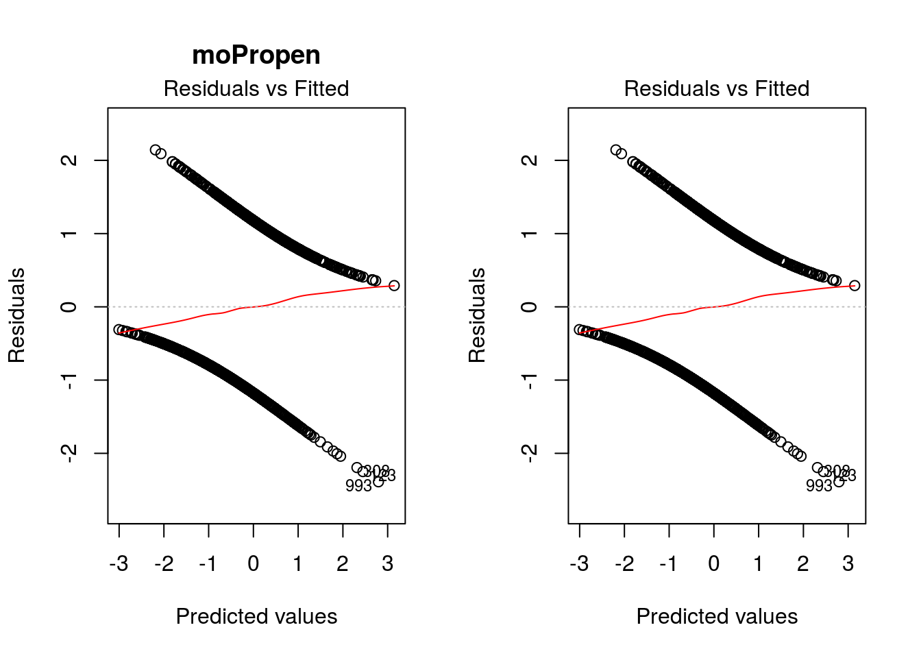
If there are additional diagnostic tools defined for a regression method used in the analysis but not implemented in DynTxRegime, the value object returned by the regression method can be extracted using function DynTxRegime::
fitObj <- DynTxRegime::fitObject(object = result)
fitObj$propensity
Call: glm(formula = YinternalY ~ SBP0 + Ch, family = "binomial", data = data)
Coefficients:
(Intercept) SBP0 Ch
-15.94153 0.07669 0.01589
Degrees of Freedom: 999 Total (i.e. Null); 997 Residual
Null Deviance: 1378
Residual Deviance: 1162 AIC: 1168As for DynTxRegime::
As such, these objects can be passed to any tool defined for these classes. For example, the methods available for the object returned by the propensity score regression are
utils::methods(class = is(object = fitObj$propensity)[1L]) [1] add1 anova coerce confint cooks.distance deviance drop1 effects
[9] extractAIC family formula influence initialize logLik model.frame nobs
[17] predict print residuals rstandard rstudent show slotsFromS3 summary
[25] vcov weights
see '?methods' for accessing help and source codeSo, to plot the residuals
graphics::plot(x = residuals(object = fitObj$propensity))
Or, to retrieve the variance-covariance matrix of the parameters
stats::vcov(object = fitObj$propensity) (Intercept) SBP0 Ch
(Intercept) 1.689875691 -8.970374e-03 -1.095841e-03
SBP0 -0.008970374 5.178554e-05 2.752417e-06
Ch -0.001095841 2.752417e-06 3.072313e-06The methods DynTxRegime::
DynTxRegime::propen(object = result)
Call: glm(formula = YinternalY ~ SBP0 + Ch, family = "binomial", data = data)
Coefficients:
(Intercept) SBP0 Ch
-15.94153 0.07669 0.01589
Degrees of Freedom: 999 Total (i.e. Null); 997 Residual
Null Deviance: 1378
Residual Deviance: 1162 AIC: 1168DynTxRegime::optimObj(object = result)$par
[1] -5.95195289 0.07819043 -1.84585674
$convergence
[1] 0
$primal
[1] 6.873585e-01 4.657276e-01 2.098597e-07 2.090176e-08 3.548702e-08 2.597633e-08 2.233927e-07 3.736546e-07
[9] 6.508203e-08 9.103840e-07 1.585779e-07 5.065093e-08 5.329653e-08 1.331259e-07 9.419309e-08 7.150605e-09
[17] 4.166505e-06 2.451895e-01 4.126304e-07 6.384030e-01 1.213346e-06 7.421093e-07 3.188540e-04 1.660435e-08
[25] 3.723721e-08 5.502811e-08 1.521397e-06 2.906062e-01 1.234600e+00 2.616232e-07 2.078862e-06 1.949988e-08
[33] 1.377899e-06 1.704358e-07 6.583618e-08 1.278381e-07 5.818292e-09 2.877724e-07 3.112444e-07 3.898919e-01
[41] 6.080201e-08 3.731499e-08 1.234016e+00 3.026224e-07 2.349471e-08 2.117663e-07 3.771155e-07 7.676579e-01
[49] 1.402218e-07 7.770047e-08 2.447324e-08 1.193817e-07 2.109766e-07 2.652043e-08 2.419361e-01 2.956444e-01
[57] 2.007566e+00 8.952383e-08 1.212272e-07 1.783887e-07 2.069556e-08 2.051909e-07 8.854774e-08 1.213956e-01
[65] 3.443066e-07 5.758897e-08 2.296620e-07 1.614263e-08 1.010191e-06 9.001008e-08 5.465592e-08 7.716575e-06
[73] 4.504214e-01 4.105532e-08 3.139420e-07 3.207152e-01 2.115536e-08 5.031630e-07 4.191346e-07 1.387080e-07
[81] 1.009760e-07 6.741525e-08 9.426781e-08 1.609942e-07 2.401899e-01 3.078331e-08 7.218755e-08 1.229551e-07
[89] 1.150433e-08 3.843732e-07 2.624840e-08 5.002716e-07 3.332174e-08 1.007825e-07 1.841894e-07 4.423597e-07
[97] 4.269108e-07 8.775123e-01 1.008913e-07 1.399191e-07 1.325353e-08 7.657675e-01 2.113652e-07 8.405020e-01
[105] 1.899729e+00 7.849705e-01 3.073995e-07 7.561195e-09 3.920434e-08 5.355789e-08 2.429055e-01 1.001327e-08
[113] 1.055387e-08 3.476640e-01 1.522210e-07 1.856143e-07 8.087729e-08 4.783231e-08 6.407030e-08 5.551324e-08
[121] 1.103223e-07 1.298068e-07 9.146226e-08 4.599872e-08 1.937838e-07 3.737391e-01 9.824179e-01 1.890062e-07
[129] 2.197990e-07 8.380133e-08 1.067846e-06 4.890011e-08 2.834195e-07 9.133550e-08 1.993639e-08 3.213284e-08
[137] 1.743094e-08 5.303950e-08 1.071213e-07 2.680215e+00 6.530522e-08 7.074195e-08 1.306294e-07 6.445486e-08
[145] 2.383151e-07 1.713289e-07 4.787099e-06 1.499342e-07 3.773466e-07 3.390760e-07 8.496281e-08 2.036393e+00
[153] 1.159271e-01 1.020253e-07 5.863334e-08 4.696707e-06 3.796426e-08 3.707052e-07 7.866520e-09 5.724967e-09
[161] 2.876636e-08 9.457850e-08 1.154967e-07 9.361321e-07 3.359718e-08 1.053854e-08 5.209815e-07 1.573687e-07
[169] 8.858625e-01 1.159540e+00 2.701209e-08 5.229191e-07 3.843212e-08 2.530816e-01 2.993768e-07 3.859216e-07
[177] 1.682591e+00 1.512326e-07 4.511568e-07 3.541330e-08 5.918697e-08 1.684681e-08 3.081187e-08 3.618906e-01
[185] 3.602399e-09 1.980486e-07 6.265602e-08 4.049043e-07 2.730509e-07 4.542376e-08 1.034638e-07 2.570641e-07
[193] 1.359806e-07 5.044406e-07 4.307877e-07 1.272964e-06 7.393991e-01 1.015936e-07 1.008803e+00 7.659671e-08
[201] 1.247344e+00 8.706447e-01 4.312979e-08 5.500373e-08 3.181642e-07 1.139013e-07 8.491951e-01 2.190497e-07
[209] 1.224720e-07 4.828662e-07 2.786405e-07 7.885727e-08 1.657196e-07 3.883132e-01 4.740318e-08 3.279984e-01
[217] 9.889558e-08 1.866263e-07 2.258705e-07 2.036516e-08 7.318116e-08 8.994932e-08 2.141308e-07 2.204953e-08
[225] 1.017511e-07 1.416423e-07 5.126205e-08 6.789397e-08 6.725313e-08 5.932355e-07 2.641446e-07 1.896262e-07
[233] 6.025501e-07 5.966258e-08 1.380627e+00 4.500994e-01 6.960957e-01 8.071710e-08 6.454767e-07 1.093965e-07
[241] 4.137886e-07 8.777559e-08 5.368864e-07 2.878393e-08 6.843325e-08 8.798473e-08 4.876075e-07 4.252305e-08
[249] 3.096315e-07 2.130615e-08 2.533092e-07 5.938165e-08 2.814338e-08 3.488389e-07 3.288034e-09 1.462901e-01
[257] 1.292754e-07 3.161178e-08 2.410613e-07 4.334246e-07 7.981722e-01 1.610175e-07 1.430659e-07 6.421181e-08
[265] 8.375636e-07 3.903546e-07 7.292234e-01 5.404489e-08 3.372590e-01 1.836401e-01 8.098317e-07 1.016665e-06
[273] 2.038637e-08 3.254489e-07 4.999089e-07 6.065168e-07 5.226484e-08 9.980448e-08 8.215213e-06 7.683939e-08
[281] 1.463244e-01 3.676859e-08 5.387761e-07 1.561945e-07 1.474458e+00 8.642274e-09 2.031766e-06 7.020824e-08
[289] 3.632058e-08 1.113766e+00 2.861946e-01 8.412463e-08 2.876387e-07 7.185515e-08 4.673837e-08 3.944163e-08
[297] 4.591509e-07 1.721668e-07 5.730146e-07 4.744248e-08 2.260506e-08 3.376173e-08 1.946338e-06 3.696072e-08
[305] 2.699923e-07 1.788756e-07 1.743880e-04 7.770028e-08 3.074811e-07 9.636017e-08 9.565548e-08 3.002968e-08
[313] 2.538893e-07 8.516500e-08 3.674329e-01 1.133171e-07 7.681132e-06 1.289241e-07 5.704532e-07 7.041705e-08
[321] 1.722245e-07 6.042577e-08 6.800660e-07 3.133810e-08 8.384960e-07 2.130714e-07 2.072157e-07 7.324829e-08
[329] 3.647962e-08 3.826971e-07 6.855322e-08 7.303106e-08 2.162475e-07 9.586212e-09 3.058225e-07 9.997964e-07
[337] 6.723491e-01 1.349436e-07 3.745573e-07 5.278044e-01 1.489182e-01 4.308673e-08 5.677844e-08 1.358964e-01
[345] 1.142706e-07 8.057411e-07 1.154594e+00 1.834590e+00 5.879699e-08 6.451155e-08 2.516054e-07 1.390065e-07
[353] 3.905464e-08 4.261568e-01 4.101508e-07 3.186498e-07 2.706097e-08 8.598716e-08 1.433706e+00 7.082746e-08
[361] 3.306412e-01 1.753665e-08 2.296895e-08 3.831677e-08 2.198413e-08 3.042134e-08 2.299755e-07 2.255817e-07
[369] 5.998238e-01 3.771508e-08 1.973796e-06 1.158096e+00 1.369851e-08 8.566207e-01 7.113651e-08 6.828303e-09
[377] 7.330050e-08 3.545464e-08 1.639491e-07 1.144939e-07 -1.013804e-08 8.680124e-07 1.923746e-07 4.164637e-07
[385] 1.873353e-08 2.610517e-07 1.692339e+00 7.110391e-08 8.993667e-09 5.581602e-08 3.244479e-08 5.453087e-07
[393] 3.799198e-08 5.740132e-08 1.903128e-07 9.742108e-07 4.629131e-06 3.248457e-08 1.129953e-01 8.691340e-08
[401] 3.433734e-08 3.597886e-07 2.225609e-09 7.849633e-08 3.165621e-01 1.582757e-08 8.213716e-08 5.411029e-07
[409] 3.687525e+00 2.876756e-08 1.240281e+00 1.014104e-08 1.193631e-07 3.796466e-01 9.479055e-08 3.258490e-08
[417] 7.482184e-08 6.512707e-08 6.783719e-08 1.033926e-07 7.053739e-07 8.299052e-01 2.417453e-07 1.178060e-01
[425] 1.760479e-07 9.147715e-08 4.418763e-09 2.113261e-06 5.709518e-07 3.684793e-07 2.343958e+00 1.323884e-07
[433] 3.510205e-09 2.176623e-07 3.356259e-07 1.266707e-07 3.200338e-08 7.164393e-07 6.211994e-07 3.660337e-07
[441] 4.350929e-07 9.382554e-07 1.084142e-07 1.728598e-07 5.014192e-01 1.737867e-07 1.709688e-07 1.746139e-08
[449] 9.349800e-09 8.889976e-01 5.499899e-01 1.293682e-07 4.457790e-07 7.826407e-01 8.262849e-08 3.310692e-01
[457] 3.877211e-08 1.003361e-07 2.582597e-08 4.843466e-08 4.864714e-01 6.730576e-07 1.328337e-07 7.297283e-08
[465] 4.049293e-07 1.623375e-07 7.189341e-07 1.630740e-08 7.180023e-08 8.216674e-08 3.508988e-01 1.049620e-06
[473] 2.184528e-01 6.835256e-08 4.912267e-07 8.247686e-08 7.405690e-08 1.142282e-07 1.613537e+00 2.264738e-07
[481] 4.999512e-08 1.294891e-06 3.595560e-07 6.173247e-01 1.254688e+00 6.158887e-08 2.106579e-07 4.900682e-07
[489] 4.691486e-08 1.026009e-07 1.580059e-07 8.711228e-08 5.066311e-01 1.161978e-07 1.490061e-07 1.069972e-07
[497] 2.948981e-08 3.306027e-07 2.437371e-08 5.795211e-07 5.888353e-07 5.664462e-01 -2.189534e-09 8.140333e-08
[505] 5.155341e-01 2.470671e-08 2.141800e-07 1.110508e-07 2.594288e-07 1.104695e-07 3.354982e-08 1.006418e-07
[513] 1.502057e-08 6.563699e-07 6.341141e-08 2.421373e+00 2.155343e-08 1.808888e-08 4.788585e-01 2.641552e-01
[521] 1.441947e+00 2.074829e-08 6.110958e-08 2.026134e-07 3.405526e-08 1.121389e+00 8.290980e-07 4.764940e-08
[529] 4.151767e-07 5.937560e-08 1.823684e-07 4.597795e-01 9.133539e-08 4.876103e-07 1.137603e-07 2.598756e+00
[537] 4.459614e-01 4.791720e-07 1.238515e-07 1.304162e+00 2.634350e-08 4.434120e-01 8.581927e-08 3.164323e-07
[545] 4.794408e-01 2.520064e+00 9.123480e-08 5.571534e-08 1.305342e-07 3.338055e-01 8.223854e-08 2.152072e-07
[553] 1.971724e+00 3.026376e-07 1.059422e-07 4.083318e-07 1.795840e-09 2.233841e-01 5.774087e-08 2.677442e-08
[561] 5.252514e-08 3.156354e-08 3.488806e-08 4.698203e-08 2.109396e-07 8.213998e-08 1.168108e-07 2.676714e-06
[569] 5.571329e-08 4.261789e-07 1.203742e-06 2.895820e+00 3.599995e-01 1.025730e+00 1.028974e-08 1.023559e-06
[577] 1.341988e-06 3.006830e-07 1.415558e-07 1.346453e-07 9.939417e-01 3.219456e-07 3.279244e-08 7.766972e-08
[585] 3.031147e-08 5.785362e-08 3.159214e-08 2.585268e+00 4.101787e-07 6.178112e-06 1.247072e-07 6.127209e-01
[593] 8.697366e-08 1.611536e-01 6.662768e-08 3.885049e-06 4.241480e-08 4.964499e-01 2.605269e-07 7.117602e-01
[601] 1.807923e-07 5.745474e-08 9.391705e-08 8.188559e-07 4.524028e-08 7.509231e-08 2.520079e-07 6.116295e-01
[609] 6.509379e-08 2.438252e-07 1.366154e-07 6.667208e-01 4.953601e-07 9.538567e-08 1.635702e-08 1.734658e-06
[617] 1.445020e+00 6.541128e-08 3.278230e-07 3.355419e-07 1.842059e-08 7.362768e-07 2.490689e-07 2.808556e-08
[625] 7.771123e-08 3.119933e-07 3.598047e-08 1.415494e+00 3.182968e+00 1.437035e-07 8.078738e-08 1.547218e-07
[633] 3.919723e-08 8.317013e-08 6.114446e-07 4.877529e-08 8.976964e-08 9.142751e-08 3.743297e-01 8.581006e-07
[641] 2.718941e-07 1.047592e-07 1.413430e+00 7.742405e-01 3.998988e-08 1.189597e-06 6.263351e-08 8.436711e-07
[649] 2.181490e-07 1.738352e-07 1.208824e-07 2.452064e-06 3.776708e-08 6.645665e-08 1.001288e-08 8.745318e-07
[657] 9.795685e-01 1.168456e-07 2.435573e-07 9.630079e-09 4.038863e-07 1.377056e-01 2.179013e-07 1.930972e-07
[665] 1.232636e-07 3.113476e-07 2.104695e+00 5.196432e-08 7.983864e-09 1.143854e-07 2.463964e-07 2.358403e-08
[673] 2.487751e-08 2.059653e-07 1.533761e-07 2.480515e-08 6.560545e-08 4.825695e-09 4.051091e-07 3.622385e-07
[681] 6.486153e-07 1.422455e-06 3.000307e-08 6.706701e-08 3.671748e-07 5.260879e-01 2.732512e-07 6.764080e-01
[689] 2.166510e-07 1.437318e-01 2.943780e-07 1.847670e-07 5.311325e-08 3.329453e-08 7.393976e-08 1.691778e-07
[697] 4.586776e-01 3.592459e-08 2.905208e-07 3.887513e-01 4.165507e-08 5.320799e-07 3.379355e-08 4.543210e-07
[705] 4.519922e-08 3.355016e-07 8.354598e-08 8.444818e-08 3.845375e-07 1.786877e-08 1.997695e-07 2.586258e-07
[713] 4.401163e-08 1.209125e-07 2.840962e-07 1.467389e-07 4.461660e-08 5.754979e-08 1.354961e-07 1.049272e-06
[721] 2.190022e-07 2.028649e-07 1.399300e-07 4.425223e-01 5.869364e-07 1.391488e+00 6.354528e-07 1.632367e-06
[729] 6.568955e-08 5.436384e-01 1.515518e+00 1.959920e-07 1.834258e-07 4.595503e-07 3.656904e-01 1.791808e-01
[737] 4.471016e-01 3.090765e-07 2.606854e-01 1.244221e-06 2.838617e-07 6.249606e-08 6.479169e-08 2.134298e-07
[745] 9.186145e-07 8.525447e-07 2.093714e-07 1.355537e-07 1.918020e-07 5.304689e-01 9.627084e-06 4.327945e-08
[753] 1.830542e-07 1.247504e-06 1.094829e-07 1.017503e-07 7.604139e-08 4.067977e-08 3.222253e-08 -3.363042e-09
[761] 4.609114e-07 3.336894e-07 3.031805e-07 2.133833e+00 5.095357e-08 8.921426e-08 5.561369e-08 6.174850e-07
[769] 3.181014e-07 7.400094e-08 1.839914e-07 5.310209e-08 1.997367e-01 1.340465e-07 3.747688e-07 1.220853e-07
[777] 1.074483e-01 5.861348e-08 5.831884e-08 1.276719e-07 1.410411e-01 8.922912e-09 3.309330e-07 1.219982e-07
[785] 3.654830e-07 4.032319e-01 6.790082e-08 5.487537e-01 4.241753e-08 3.705241e-06 5.272427e-07 2.632791e-07
[793] 1.193745e-07 2.754786e-01 -4.900252e-09 2.979878e-08 5.455916e-08 2.940090e-07 7.834515e-07 1.391337e-07
[801] 8.163452e-08 4.818111e-07 4.322973e-01 1.501063e-08 1.352322e-07 8.593610e-05 1.470356e-07 6.062334e-08
[809] 3.109329e-08 2.208525e-07 4.292292e-07 1.164323e-07 1.127425e-07 1.510180e-07 1.470946e-07 2.748969e-07
[817] 4.451006e-07 2.889014e-08 1.971511e-07 5.143320e-08 1.270230e-06 1.895477e-07 2.125291e-07 4.470975e-07
[825] 1.204660e-01 2.669378e-07 2.193694e-01 1.213705e-08 4.206971e-07 9.298415e-08 4.854122e-07 3.961066e-01
[833] 1.824884e-01 1.707186e-07 2.143349e-07 5.971724e-08 4.646514e-08 1.548686e-07 4.851620e-07 6.508764e-01
[841] 4.038564e-08 5.293837e-07 1.679798e+00 3.140258e-07 1.074345e+00 7.470789e-08 1.892524e-07 1.543159e-07
[849] 8.139681e-01 7.447597e-08 2.109826e-07 3.958941e-01 3.418386e-08 1.676156e-07 2.047953e-07 3.960913e-08
[857] 8.236840e-08 3.783033e-08 3.599950e-07 6.839722e-08 6.148045e-08 5.553946e-01 7.456799e-07 7.739811e-07
[865] 2.745355e-07 1.306883e-06 4.300102e-07 6.557452e-01 1.350349e-01 4.114247e-06 2.922864e-01 1.408298e+00
[873] 1.423651e-08 7.508628e-01 4.531144e-08 4.823204e-01 1.226541e-07 1.129539e-01 6.819238e-01 8.072283e-08
[881] 1.195309e-06 1.333791e-07 8.883275e-08 1.808587e-06 1.705017e-07 1.475469e-07 5.408592e-08 3.394542e-01
[889] 1.778332e-08 5.467128e-08 1.068669e-06 3.771238e-07 3.293815e-01 4.614764e-08 2.747891e-07 1.366768e-07
[897] 3.749879e-08 3.472459e-08 5.311349e-08 1.083982e-07 1.287031e-06 6.113494e-08 7.399304e-01 9.367485e-08
[905] 1.537134e-06 1.455671e-07 1.636800e+00 2.375161e-07 7.554317e-09 2.635233e-08 3.303537e-08 1.280710e-06
[913] 3.120432e-08 5.818400e-08 1.181099e-06 6.098475e-01 2.552638e-06 4.318453e-08 8.833119e-01 8.392670e-07
[921] 3.059747e-06 6.885577e-08 1.020843e+00 2.537754e-07 1.351515e-07 4.693853e-01 8.038710e-08 3.157276e-07
[929] 9.230125e-09 4.174676e-01 7.297479e-08 1.213578e-07 1.333249e-07 1.581908e-07 1.494692e-07 2.059006e-07
[937] 1.170663e-07 7.064881e-07 2.956070e-07 5.250487e-01 4.527768e-08 8.001877e-01 5.798388e-08 5.846035e-01
[945] 2.958631e-08 4.688706e-06 5.929633e-05 3.954180e-07 1.515360e-07 6.775558e-08 1.677363e-08 5.789683e-08
[953] 5.511922e-07 2.618725e-07 2.221274e-07 5.841810e-08 5.107327e-08 1.831757e-08 2.556363e-06 8.661531e-07
[961] 3.163963e-07 2.810404e-01 5.830837e-07 9.382909e-01 2.950558e-07 8.095274e-08 7.887000e-08 4.818927e-08
[969] 3.677421e-01 1.070300e-06 1.509965e-07 5.015290e-01 6.696446e-08 2.207556e-07 2.234879e-07 1.005819e-07
[977] 1.779241e-07 1.606217e-07 2.439924e-08 1.785989e-07 5.994683e-01 4.591753e-08 -2.925075e-09 4.439151e-01
[985] 5.509332e-08 2.070190e-07 1.112365e-01 2.438130e-07 1.728881e-07 5.538897e-08 3.318641e-08 8.620891e-08
[993] 3.034349e-07 3.912315e-07 6.993638e-08 3.756927e-07 2.409209e-07 8.247482e-07 2.791108e-07 3.524515e-07
$dual
[1] 5.951953
$how
[1] "converged"
$lambda
[1] 0.1
$surrogate
[1] "HingeSurrogate"
$kernel
[1] "linear"
$kernelModel
~Ch + K - 1Once satisfied that the postulated model is suitable, the estimated optimal treatment regime, the recommended treatments, and the estimated value for the dataset used for the analysis can be retrieved.
The estimated optimal treatment regime is retrieved using function DynTxRegime::
DynTxRegime::regimeCoef(object = result)[1] -5.95195289 0.07819043 -1.84585674Function DynTxRegime::
DynTxRegime::optTx(x = result)$optimalTx
[1] 1 0 1 1 1 1 1 0 1 1 1 1 1 0 0 1 0 0 0 1 1 1 0 1 1 1 1 1 1 1 1 1 0 1 1 1 1 1 0 0 1 1 1 0 1 1 1 0 1 1 1 1 1 1 1 1 1 1 1
[60] 1 1 1 1 1 1 1 1 1 1 1 1 1 1 1 1 0 1 0 1 1 0 1 1 1 0 1 1 1 1 1 1 1 1 1 1 1 1 1 1 1 1 1 1 0 1 1 1 1 1 1 0 1 1 1 1 1 0 1
[119] 1 1 1 1 1 1 1 0 1 0 1 1 1 1 1 0 1 1 1 1 0 1 1 1 1 1 0 1 1 1 0 1 1 1 1 1 1 0 1 1 1 1 1 1 1 0 1 1 1 1 1 1 1 0 1 0 1 1 1
[178] 1 1 1 1 1 1 1 1 0 1 1 0 1 1 1 1 1 1 1 0 1 1 1 0 0 1 0 1 1 0 1 1 0 0 0 1 1 1 0 1 1 1 1 1 1 1 1 1 1 1 0 1 1 1 1 1 0 1 1
[237] 1 1 1 0 1 0 1 0 1 1 1 1 0 1 1 1 1 1 1 1 1 1 0 0 0 0 1 1 0 1 1 0 1 1 1 1 1 0 1 1 1 1 0 1 1 1 0 1 0 1 0 1 1 1 0 1 1 1 1
[296] 1 1 1 1 1 1 1 1 1 1 1 0 1 1 0 1 1 1 1 1 0 0 1 0 1 1 1 0 1 1 0 1 1 1 1 1 1 1 1 1 1 0 1 1 0 1 1 1 1 1 1 1 1 1 1 0 1 1 1
[355] 1 0 1 1 1 1 1 1 1 1 1 1 1 0 1 1 0 0 1 0 1 1 1 1 1 1 1 0 1 0 1 1 1 1 1 0 0 1 0 1 1 0 1 1 1 1 1 1 1 1 1 1 1 0 0 1 0 1 1
[414] 1 1 1 0 1 1 1 1 1 1 1 1 1 1 1 1 1 1 1 1 1 1 1 1 1 0 1 0 1 1 0 1 1 1 1 1 1 1 0 0 0 1 1 1 1 1 1 1 1 0 1 1 1 1 1 1 1 1 1
[473] 0 1 1 1 0 1 1 1 1 1 1 0 1 0 1 1 1 1 1 1 1 1 0 0 1 1 1 1 0 0 1 0 0 1 1 0 1 1 1 0 1 1 1 0 1 1 1 0 0 1 1 1 1 1 1 1 0 1 0
[532] 0 1 1 1 0 1 1 1 1 1 0 0 1 0 1 1 1 1 0 1 1 1 0 1 0 1 0 1 1 1 1 1 1 1 1 1 1 1 0 1 0 0 1 1 0 1 1 1 0 1 0 1 1 1 1 1 0 0 1
[591] 1 0 1 1 1 1 1 0 1 1 1 1 1 1 1 1 1 0 1 0 0 1 0 1 1 1 1 1 0 0 1 1 1 1 1 0 1 0 0 0 0 1 1 0 0 1 1 1 1 1 0 1 0 0 1 1 1 1 1
[650] 1 1 1 1 1 1 0 1 1 1 1 1 1 1 1 1 0 1 1 1 1 0 1 1 1 1 1 1 1 0 0 1 0 1 1 1 1 0 0 0 0 1 1 1 1 1 0 0 1 1 1 1 1 1 1 1 1 1 1
[709] 1 1 1 1 1 1 1 0 1 0 1 0 1 1 0 1 0 0 1 1 1 0 1 1 0 1 1 0 1 0 0 1 1 0 0 1 0 1 1 1 1 1 0 1 1 0 0 1 1 1 1 1 0 0 0 1 1 1 1
[768] 0 1 1 1 1 0 1 1 1 0 1 1 1 1 1 1 1 1 1 0 0 1 1 0 0 1 0 1 1 1 1 0 1 1 1 0 1 1 1 1 1 1 0 0 1 1 0 1 0 1 1 1 1 0 1 0 1 0 0
[827] 0 1 1 1 1 1 1 1 1 1 1 1 1 1 1 1 1 0 1 1 0 1 1 1 1 1 1 1 1 1 1 1 1 1 1 1 1 0 1 1 1 1 1 1 1 1 1 0 1 0 1 1 1 1 1 0 1 1 1
[886] 1 0 1 1 1 0 1 0 1 1 1 1 1 0 1 1 1 0 1 0 1 0 1 1 1 1 0 1 1 1 1 1 1 0 1 0 1 0 0 0 1 1 0 1 1 1 1 1 1 1 1 1 1 1 0 1 1 1 1
[945] 1 0 1 1 1 1 1 1 1 1 0 1 1 1 1 0 1 1 0 1 1 1 1 1 1 0 1 1 1 1 1 1 0 1 1 0 1 1 1 1 1 0 0 1 0 1 1 0 1 0 0 0 1 1 1 1
$decisionFunc
[1] 0.33091158 -0.43731229 3.02848127 9.71822903 6.55654582 7.31806430 2.89388120 -2.30131577 5.10331756
[10] 1.51270066 3.38619954 5.81792178 5.77128887 -3.73191922 -4.42949035 9.89834835 -1.14716882 -0.50907867
[19] -0.77017843 0.49790147 1.42557754 1.70873942 -1.00810240 8.43758239 6.70957398 5.49287468 1.34571077
[28] 0.38201084 0.42110605 2.66852396 1.24238687 8.08097778 -1.36470701 3.27366159 5.13459373 3.74001414
[37] 11.00501836 2.56073372 -2.44205854 -0.04468381 5.35799327 6.60122104 0.44763453 -2.58587265 7.68053026
[46] 2.98128567 2.20552411 -0.77185477 3.65400468 4.89555610 7.47276881 3.96034234 2.93409007 7.42250186
[55] 0.07874452 0.35408736 0.35548236 4.35464716 3.90560904 3.21585695 7.96508714 3.00167145 4.51856571
[64] 3.20468521 2.30717166 5.37084135 2.83272386 8.59368190 1.52415375 4.35101312 5.58474550 1.09075371
[73] 0.96397268 6.19519352 2.44177173 -0.09634576 7.89024941 -1.97598733 2.13543407 3.63808525 -4.29349528
[82] 4.99692231 4.54648919 3.47667535 -0.69226935 6.92683083 4.97207018 3.82071323 9.13822488 2.18374332
[91] 7.40797743 1.94610070 6.76905497 4.25886096 3.21920964 2.11365329 2.11811964 0.02904026 4.07762798
[100] 3.57999925 8.64813385 0.48868743 2.96732393 -0.70623108 1.01423963 0.08042087 2.50767676 10.99440932
[109] 6.37475015 5.61630302 -0.59062179 9.60094339 9.48505275 0.94554459 3.33621393 3.12342344 -4.64228085
[118] 6.05109806 0.01479718 5.48645064 3.97569908 3.70203259 4.90002245 5.92292203 2.95279950 -0.83301211
[127] 0.28232098 -0.47165981 2.96285758 4.61267557 1.45517736 5.77268387 2.56073372 -4.47361461 8.15553417
[136] 6.97039239 8.44344374 5.68025036 -4.19994812 0.93688151 5.10974160 5.06450369 3.70482259 5.10192256
[145] -2.80452450 3.32867624 1.12174853 3.51465691 -2.20581091 2.31359570 4.47611780 0.44791587 0.05053970
[154] 4.22451344 5.43311235 -1.11449764 6.56854987 2.18513833 9.85143410 10.56575697 7.13794498 4.35771851
[163] 3.96173734 -1.56325442 6.71711168 9.41803406 1.79586254 3.16419500 0.05975374 0.49036378 6.92822583
[172] -1.96342059 6.53420235 -1.04998761 2.54202428 2.23875797 0.50264917 3.47695670 2.09466251 6.70957398
[181] 5.51297912 8.29181058 7.10666880 0.95587229 10.52694311 -3.10360581 5.28147919 2.19016737 -2.68919655
[190] 5.98212167 4.11169415 2.67159531 3.70706163 1.99776265 2.09159116 1.35939116 -0.60597853 4.25914230
[199] 0.79027740 4.71850812 -1.17258364 -0.86428828 6.09326462 -5.56185653 2.43255769 3.87377018 -0.80452594
[208] 2.89527620 3.92878482 -1.88187747 -2.63139191 -4.81122844 3.34570932 0.89192495 5.93856011 -3.14995737
[217] 4.19156092 3.17061904 2.81680443 7.92152558 4.85617954 4.48086550 2.94219046 7.76989242 4.21194670
[226] 3.65400468 5.66964132 -0.17118349 5.07343639 1.85255353 2.66712896 3.16140499 1.80368159 -6.16085146
[235] 0.54453438 1.76793907 1.22479109 4.65288443 1.74112925 -4.13264808 2.19016737 -4.59061890 1.90393414
[244] -7.04161327 5.09103216 4.45908472 1.95531474 6.15470330 -2.60318708 7.77631646 2.70287148 5.36330365
[253] 7.30689256 2.32448609 11.52135652 0.17760207 3.58921330 6.87042118 -2.89277300 -1.95085386 -0.15247406
[262] -3.50265833 3.64590429 5.16279855 -1.65875928 2.19323871 0.50293051 -0.80005959 0.50432552 0.64813963
[271] 1.59563878 1.48505853 7.97793523 -2.49539683 1.96481013 1.76598137 5.63668880 1.03266772 -1.07847378
[280] 4.76263238 0.96843903 6.51688792 -1.87126843 3.37223780 -0.97403622 10.35185282 -1.19547807 4.97793153
[289] 6.55151678 0.55459246 -0.39961208 4.51214167 2.49315233 0.23512537 5.89164586 6.32029820 1.95978109
[298] 3.30968546 1.86483893 5.99329341 7.79139186 6.75034554 1.26584399 6.65288299 2.58083815 3.21418060
[307] -1.01117374 5.35687961 2.44959077 -5.34738968 4.24154653 7.04244012 2.72493361 4.56519862 0.24433942
[316] -4.09048152 -1.08322147 3.78832340 -1.93242577 5.27561784 3.17340904 5.27198380 -1.76962087 6.89862600
[325] 1.59899148 -2.96872439 3.00949049 4.99552731 6.68415916 2.23401027 4.98296057 4.83914646 2.93130006
[334] 10.21222371 2.50432407 1.44093428 -0.11673154 3.77910936 2.22283854 -0.49818828 0.13990186 6.09465962
[343] 5.45238447 2.19212506 4.02457103 1.60345783 0.48198204 0.98714846 2.25439605 5.18486068 -2.81597758
[352] 3.63026620 6.34179763 1.77072907 2.09438116 -2.35633041 7.28957813 4.51381801 0.98156846 4.91398419
[361] 0.68248715 8.19686842 7.74308260 6.40434997 7.71990682 6.94721661 2.85618099 -2.87182453 0.21334459
[370] 6.49203579 -1.26166445 -0.44373633 8.81289643 -0.92544562 4.89527475 9.99999591 4.87684667 6.85031675
[379] 3.36134741 3.96034234 12.65679404 -1.55822538 3.08265188 -2.18403013 8.14185377 2.65288588 0.99664385
[388] 4.95782710 9.84947641 -5.21670500 -6.84557451 1.82546237 -6.34711348 5.47081256 3.16140499 -1.52555421
[397] 1.12649623 6.79865480 0.92794882 4.53113245 6.80312115 2.27729049 11.00529971 4.80647528 0.94219190
[406] 8.58753920 4.66098482 -1.90226325 -0.11226519 7.20524501 -0.28567913 9.46187697 3.91649943 0.66992041
[415] 4.35436582 6.91565909 -0.39821707 5.13934142 5.05807965 4.15442340 1.72102481 1.10806814 2.79055730
[424] 0.77631566 3.17508539 4.42948489 11.36190432 1.24545821 1.85227219 2.25411471 0.67103407 3.62691351
[433] 11.07567109 2.88103312 2.39346247 3.76821897 7.00473991 1.67075786 -1.76487318 2.28706723 -2.12790183
[442] 1.52219605 3.94274656 -3.31779131 0.55570612 3.28483333 3.27366159 8.27031115 8.47695895 0.05835874
[451] 1.25299591 -3.18486758 -2.07456354 -0.94080236 4.69868503 0.57162555 6.48589309 4.19798496 7.40993512
[460] 5.94135011 2.04579056 1.73023885 -2.89249166 4.83914646 2.15553850 3.38927088 1.66601017 8.49538704
[469] 4.85617954 4.54648919 0.15246860 1.43925793 -0.37168860 4.97653653 1.96173878 4.58558440 -4.90840964
[478] 3.97290908 0.41552605 2.73247131 5.84166025 1.37698694 2.22423354 -0.71684013 0.14604456 -5.28232869
[487] 2.99245740 1.98212456 5.89611221 4.21194670 3.46159996 4.46997511 0.23373037 3.94945195 -3.60570088
[496] -4.20944351 7.03183107 2.33677148 7.57413501 1.82239102 -1.86959208 -0.74225495 8.04327757 -4.71768127
[505] -1.25384541 7.48980189 2.98463836 -3.86987198 2.66098627 3.99608486 6.91594043 -1.41636896 8.77659122
[514] 1.63920035 5.15665585 -0.61743161 7.86679228 8.23121594 0.83886800 -0.09327441 -0.61882661 7.94470136
[523] 5.23177493 2.97486163 6.84249770 0.16307764 1.66293882 5.87740277 -2.13376318 5.44596043 -3.26166301
[532] -0.43256459 4.38257064 1.95224340 3.96620369 -0.85311655 2.56408641 1.95531474 3.82574227 0.52471130
[541] 11.27896620 -0.77967381 -0.52164541 2.41831460 -1.00167835 0.60262038 4.47332780 5.45852717 3.67997046
[550] -0.81430268 4.54677053 2.96118123 1.57442069 -2.56883957 4.01647064 -2.19184917 11.38982779 -0.16196945
[559] 5.40965522 6.82657827 5.99301206 6.87516888 6.71236398 5.86958373 2.96871893 4.57162266 3.87405152
[568] 1.20971570 5.49315603 -2.17313974 1.42222485 -0.38369265 -0.53114080 0.77799201 9.96508570 -1.45685917
[577] 1.41887215 2.53281024 3.63361890 -3.77297212 0.99999655 -2.50963992 6.83300231 4.67215656 6.55291178
[586] 5.77128887 7.01870164 -0.55013158 -2.22647804 1.10778680 3.85087574 -0.71712147 4.98463692 0.80144913
[595] 5.03797521 1.14688201 6.32141185 -0.40128842 2.67801935 0.43534913 3.17033769 5.47081256 4.25718461
[604] 1.56632031 6.05416940 4.78134181 2.69812379 -0.92069793 5.08293178 -2.82212028 -3.70231939 0.64478694
[613] -1.83831591 4.20273266 8.50934878 1.30186786 0.59451999 5.06729369 -2.40742967 -2.40910602 8.32922945
[622] 1.67885825 2.75006708 7.20664001 4.77631277 -2.42753411 6.72185937 -0.34069377 -0.16671715 -3.65568648
[631] -4.13404308 3.46774266 6.50320752 -2.86568184 -1.82714418 5.81177908 4.49678493 4.30577521 0.12901147
[640] 1.52862009 -2.64702999 4.16028475 -0.25468431 -0.17760754 6.33286493 1.40044407 5.25495071 1.58167705
[649] 2.83411886 3.22507099 3.84249401 1.20943435 6.41384536 5.03937021 9.77603367 -1.61324002 0.40853931
[658] 4.01172294 2.79390999 7.12091189 2.19184371 0.87461052 2.95029084 2.75620978 3.85255209 -2.48757779
[667] 0.30689176 5.96955494 8.98491537 4.00250890 -2.80955354 7.64450640 7.56659732 2.84529060 3.43143744
[676] 7.44149263 5.24238398 7.02065934 -2.22312534 -2.27478729 1.65204843 -1.37420240 6.98491682 5.08767947
[685] 2.21334315 0.18988747 -2.71712003 -0.65652683 -2.97542978 -0.44680768 2.55459102 3.13934287 5.86847007
[694] 6.94079256 4.87852301 -3.30326688 -0.40603612 6.54705043 2.53727659 0.87321552 6.24182643 1.88801471
[703] 6.76430728 2.06813403 6.02317458 2.38731978 4.59200844 4.51074667 2.02568613 8.24685402 3.08460957
[712] 2.63054241 6.04160267 3.93353252 2.57804815 -3.65122014 6.00390245 -5.48701880 4.33537504 -1.50684477
[721] 2.92040967 3.05026205 -3.63837205 0.87182052 -1.88690651 -0.98296892 1.69728634 1.30493921 5.19714607
[730] -0.23373583 0.57944459 3.11113804 -3.18933393 2.01479574 1.00278655 -0.37615495 0.66992041 -2.43088680
[739] -0.51243137 1.40183907 2.62049605 -0.16364580 -5.13655688 2.89359985 -1.53030190 1.55654357 2.95782854
[748] 3.65511833 3.14101921 0.24601577 -1.07065474 6.08376923 3.18932847 -1.43340204 -4.15917656 4.41998950
[757] 4.72521351 6.23233104 7.00194990 11.66070428 -2.10276836 -2.42195410 -2.48422510 0.16000630 5.68360305
[766] 4.41691816 5.48002660 -1.82267783 2.38536209 4.85953224 3.15637595 5.59395955 -0.89249310 3.69086085
[775] 2.23344758 3.86316113 -2.01954889 5.37223635 5.34263653 3.80870918 2.68137205 9.45266293 2.28231953
[784] 3.68639450 2.32337244 1.43758159 -5.16112766 -0.49344059 6.20719756 1.14520566 -1.92600173 -2.67970116
[793] 3.84445170 -0.62636431 11.87935613 7.10974015 5.50180738 2.50097138 -1.70874488 3.44093283 4.66852252
[802] 1.90365279 -0.41385516 8.63920115 3.68639450 1.00921059 3.55375212 5.27701284 7.10834515 -2.91399109
[811] -2.09634432 3.85841344 3.97402273 -0.68752165 3.50655652 -2.61072478 2.09019616 6.76737863 3.04690936
[820] 5.64450784 -1.41636896 3.10164265 -2.24797747 1.96452879 -0.43395959 -2.66071038 -0.51857406 9.32867190
[829] 2.16531524 1.07343928 2.03239151 0.12258743 0.21027325 3.30354276 2.96900028 5.46466986 5.90114125
[838] 3.43450879 1.95531474 2.51493312 6.52638331 1.85673854 1.28091939 -2.43228180 0.38732122 4.86902762
[847] -3.19911067 3.48980478 0.40379162 4.84193646 2.84947560 2.20915814 6.66265972 3.30326142 2.99692375
[856] 6.38396419 4.57190401 6.45126423 2.25411471 5.02987483 5.26109341 0.83272530 1.58474839 -1.62077772
[865] 2.59508123 1.37559194 2.11504829 0.66684906 0.91063438 1.14073931 0.61993481 0.52275360 8.70203484
[874] -0.54510254 5.96815994 -0.75956938 3.88047557 0.14157821 0.30131175 4.72660851 1.35939116 -3.79978194
[883] 4.42752720 1.29097747 3.28622833 3.50655652 -1.10639726 0.97039672 8.31387271 5.52889855 -1.14995882
[892] 2.23708162 -2.15610665 5.91482164 2.58558584 1.95391974 6.72046437 6.70314994 -5.46020897 3.99273216
[901] 1.38620098 5.28008419 -0.35437417 4.26807500 -1.36331201 3.53476135 -1.00000201 2.69812379 10.13570963
[910] 7.43199725 6.84417405 -1.41944031 6.85310675 5.81177908 1.41608215 1.81317698 1.20496800 6.07930288
[919] -0.24797892 1.58949609 -1.17062594 4.98128422 -1.02317779 -2.81458258 -3.71684382 0.20384920 4.72521351
[928] -2.55320148 9.48561544 2.59787124 0.66042502 3.92767117 3.68639450 3.40351397 3.50041383 2.99385241
[937] 3.94609925 1.64087669 2.51856715 -0.46160173 5.98658802 2.00586304 5.37223635 0.70594428 7.05807820
[946] -1.12706438 1.01870598 2.12733368 3.48812844 5.04076522 8.43897739 5.36441731 1.87237662 2.67327166
[955] -2.87964358 5.36162731 5.66182227 8.01200140 1.20496800 -1.60849233 2.23512393 0.28539232 -1.81346378
[964] 0.12426378 2.53252889 4.66405617 4.64674174 6.11839809 1.62523861 -1.41301626 3.47220900 2.63221875
[973] 0.71208697 2.95029084 2.91426698 4.13543262 -2.19352552 3.39262358 7.51325902 -3.29126283 0.59647768
[982] 5.95252185 12.47053202 0.38201084 5.49901738 -3.02848673 -0.72661686 2.72632861 -3.31779131 5.63529380
[991] 6.87628253 -3.60402453 8.66126328 -2.29377807 -1.29098293 -2.33594463 2.74029035 1.59424378 2.57469545
[1000] 2.33091013The object returned is a list. The element names are $optimalTx and $decisionFunc, corresponding to the \(\widehat{d}^{opt}_{\eta}(H_{1i}; \widehat{\eta}_{1})\) and the estimated decision functions, respectively. Note that the estimated optimal treatment is returned as provided in the original data, i.e. \(\{0,1\}\), rather than the sign of the decision function \(\{-1,1\}\).
Function DynTxRegime::
DynTxRegime::estimator(x = result)[1] 13.07951Function DynTxRegime::
The first new patient has the following baseline covariates
print(x = patient1) SBP0 W K Cr Ch
1 162 72.6 4.2 0.8 209.2The recommended treatment based on the previous analysis is obtained by providing the object returned by DynTxRegime::
DynTxRegime::optTx(x = result, newdata = patient1)$optimalTx
[1] 1
$decisionFunc
[1] 2.652886Treatment A= 1 is recommended.
The second new patient has the following baseline covariates
print(x = patient2) SBP0 W K Cr Ch
1 153 68.2 4.5 0.8 178.8And the recommended treatment is obtained by calling
DynTxRegime::optTx(x = result, newdata = patient2)$optimalTx
[1] 0
$decisionFunc
[1] -0.2778601Treatment A= 0 is recommended.
Residual Weighted Learning
For the residual weighted learning (RWL) method, one minimizes in \(\eta_{1}\) the weighted classification error
\[ \begin{align} & n^{-1} \sum_{i=1}^{n} \left[ \frac{Y_i - \widehat{g}^*(H_{1i}; \widehat{\beta}_{1})}{\pi_{d_{\eta},1}(H_{1i};\eta_{1}, \widehat{\gamma}_{1})} \text{I}\{ A_{1i} \neq d_{1}(H_{1i}; \eta_{1})\} \right], \end{align} \]
where \(\widehat{g}^*(h_{1}; \widehat{\beta}_{1})\) is obtained by positing a linear model directly for the main (common) effects of clinical covariates for both treatment arms and fitting it using a version of weighted least squares. As for OWL, writing \(d_{1}(H_{1}; \eta_{1})\) in terms of a decision function \[ \widehat{d}^{opt}_{\eta,RWL} = \{ d_{1}(h_{1}; \widehat{\eta}^{opt}_{1,RWL}) \} = \text{I}\{ f_1(h_{1}; \widehat{\eta}^{opt}_{1,RWL}) \gt 0\}, \] implementation is accomplished by replacing the nonconvex 0-1 loss function by a smooth surrogate loss function. Specifically,
\[ T(u) = \left\{ \begin{align} &0 & \text{if} &~ u >= 1,\\ &(1-u)^2 & \text{if}&~ 0 \le u < 1\\ &2 - (1-u)^2 & \text{if}&~-1 \le u < 0\\ &2 & \text{if}&~u < -1. \end{align} \right. \]
Such that the estimator is reexpressed in the regularization framework as \[ \begin{align} \min_{\eta}~~& n^{-1} \sum_{i=1}^{n} \left[ \frac{Y_i - \widehat{g}^*(H_{1i}; \widehat{\beta}_{1})}{ \pi_{d_{\eta},1}(H_{1i};\eta_{1}, \widehat{\gamma}_{1})} T\left\{A_{1i} f_{1}(H_{1i};\eta_{1})\right\} \right] + \frac{\lambda}{2} ||f||^2, \end{align} \]
The smoothed ramp loss is a non-convex loss, and the optimization problem involves non-convex minimization. The authors apply the Difference of Convex (d.c.) algorithm to solve this non-convex minimization problem, which assumes that an objective function can be rewritten as the sum of a convex part, \(Q_{vex}(\Theta)\), and a concave part, \(Q_{cav}(\Theta)\). The non-convex optimization problem is solved by minimizing a sequence of convex subproblems. The details of this method are beyond the scope of this presentation; we refer the readers to the original manuscript for further details.
A general implementation of the RWL estimator is provided in
utils::str(object = DynTxRegime::rwl)function (..., moPropen, moMain, data, reward, txName, regime, response, fSet = NULL, lambdas = 2, cvFolds = 0L, kernel = "linear",
kparam = NULL, responseType = "continuous", verbose = 2L) We breifly describe the input arguments for DynTxRegime::
| Input Argument | Description |
|---|---|
| \(\dots\) | Used primarily to require named input. However, inputs for the optimization methods can be sent through the ellipsis. |
| moPropen | A “modelObj” object. The modeling object for the propensity score regression step. |
| moMain | A “modelObj” object. The modeling object for \(g(h_{1}; \beta_{1})\). |
| data | A “data.frame” object. The covariate history and the treatment received. |
| reward | A “numeric” vector. The outcome of interest, where larger values are better. This input is equivalent to response. |
| txName | A “character” object. The column header of data corresponding to the treatment variable. |
| regime | A “formula” object or a character vector. The covariates to be included in classification. |
| response | A “numeric” vector. The outcome of interest, where larger values are better. |
| fSet | A “function”. A user defined function specifying treatment or model subset structure. |
| lambdas | A “numeric” object or a “numeric” vector. One or more penalty tuning parameters. |
| cvFolds | An “integer” object. The number of cross-validation folds. |
| kernel | A “character” object. The kernel of the decision function. Must be one of {linear, poly, radial} |
| kparam | A “numeric” object, a “numeric” “vector”, or NULL. The kernel parameter when required. |
| responseType | A “character” object. Indicates if response/reward is binary, continuous, or count data. qMust be one of {continuous, binary,count}. |
| verbose | A “numeric” object. If \(\ge 2\), all progress information is printed to screen. If =1, some progress information is printed to screen. If =0 no information is printed to screen. |
Though the RWL method has was developed in the original manuscript in the notation of \(\mathcal{A} \in \{-1,1\}\), this is not a requirement of the implementation in DynTxRegime. It is only required that treatment be binary and coded as either integer or factor.
The value object returned by DynTxRegime::
| Slot Name | Description |
|---|---|
| @responseType | The type of the response variable. |
| @residuals | The residuals of outcome regression analysis. |
| @beta | The betas of d.c. algorithm. |
| @analysis@txInfo | The treatment information. |
| @analysis@propen | The propensity regression analysis. |
| @analysis@outcome | The outcome regression analysis. |
| @analysis@cvInfo | The cross validation results. |
| @analysis@optim | The final optimization results. |
| @analysis@call | The unevaluated function call. |
| @analysis@optimal | The estimated value, decision function, and optimal treatment for the training data. |
There are several methods available for objects of this class that assist with model diagnostics, the exploration of training set results, and the estimation of optimal treatments for future patients. We explore these methods under the Methods tab.
We continue to consider the propensity score and outcome models introduced in Chapter 2, which represent a range of model (mis)specification. For brevity, we discuss the function call to DynTxRegime::
Input moPropen is a modeling object for the propensity score regression. To illustrate, we will use the true propensity score model
\[ \pi^{3}_{1}(h_{1};\gamma_{1}) = \frac{\exp(\gamma_{10} + \gamma_{11}~\text{SBP0} + \gamma_{12}~\text{Ch})}{1+\exp(\gamma_{10} + \gamma_{11}~\text{SBP0}+ \gamma_{12}~\text{Ch})}, \] which is defined as a modeling object as follows
p3 <- modelObj::buildModelObj(model = ~ SBP0 + Ch,
solver.method = 'glm',
solver.args = list(family='binomial'),
predict.method = 'predict.glm',
predict.args = list(type='response'))We will use the main effects component of the correctly specified outcome regression model \(Q^{3}_{1}(h_{1},a_{1};\beta_{1})\). Specifically,
q3Main <- modelObj::buildModelObj(model = ~ (Ch + K),
                                  solver.method = 'lm',
predict.method = 'predict.lm')As for all methods discussed in this chapter: the ‘data.frame’ containing the baseline covariates and treatment received is data set dataSBP, the treatment is contained in column $A of dataSBP, and the outcome of interest is the change in systolic blood pressure measured six months after treatment, \(y = \text{SBP0} - \text{SBP6}\), which is already defined in our R environment.
The outcome of interest can be provided through either input response or input reward. This “option” for how the outcome is provided is not the standard styling of inputs for
The decision function \(f_{1}(H_{1};\eta_{1})\) is defined using a kernel function. Specifically,
\[ f_{1}(H_1;\eta_{1}) = \sum_{i=1}^{n} \eta_{i} A_{1i} k(H_1,H_{1i}) + \eta_0 \]
where \(k(X,X_{i})\) is a continuous, symmetric, and positive definite kernel function. At this time, three kernel functions are implemented in DynTxRegime:
\[ \begin{array}{lrl} \textrm{linear} & k(x,y) = &x^{\intercal} y; \\ \textrm{polynomial} & k(x,y) = &(x^{\intercal} y + c)^{\color{red}d}; ~ \textrm{and}\\ \textrm{radial basis function} & k(x,y) = &\exp(-||x-y||^2/(2 {\color{red}\sigma}^2)). \end{array} \]
Notation shown in \(\color{red}{red}\) indicates the kernel parameter that must be provided through input kparam. Note that the linear kernel does not have a kernel parameter.
For this illustration, we specify a linear kernel and will include baseline covariates Ch and K in the kernel. Thus,
kernel <- 'linear'
regime <- ~ Ch + K
kparam <- NULLWe do not illustrate the cross-validation capability here, but refer the reader to the discussion of the outcome weighted estimator for an example of its use. We specify \(\lambda_{n} = 0.01\), and thus cvFolds = 0.
Circumstances under which this input would be utilized are not represented by the data sets generated for illustration in this chapter.
The optimal treatment regime is estimated as follows.
RWL33 <- DynTxRegime::rwl(moPropen = p3,
moMain = q3Main,
data = dataSBP,
reward = y,
txName = 'A',
regime = regime,
lambdas = 0.01,
cvFolds = 0L,
kernel = kernel,
kparam = kparam,
responseType = 'continuous',
verbose = 1L)Residual Weighted Learning
Propensity for treatment regression.
Regression analysis for moPropen:
Call: glm(formula = YinternalY ~ SBP0 + Ch, family = "binomial", data = data)
Coefficients:
(Intercept) SBP0 Ch
-15.94153 0.07669 0.01589
Degrees of Freedom: 999 Total (i.e. Null); 997 Residual
Null Deviance: 1378
Residual Deviance: 1162 AIC: 1168
Outcome regression.
moMain only outcome regression model. ~(Ch + K)
Regression analysis for moMain:
Call:
lm(formula = YinternalY ~ Ch + K, data = data)
Coefficients:
(Intercept) Ch K
-53.59368 0.08271 9.61264
Final optimization step.
current max beta diff: 0.00310353
current max beta diff: 0.01254147
current max beta diff: 0.002589314
current max beta diff: 0.01139547
current max beta diff: 0.001635163
current max beta diff: 0.008941053
current max beta diff: 0.00207367
current max beta diff: 0.002346253
current max beta diff: 0.001922428
current max beta diff: 0.009393359
current max beta diff: 0.001332459
current max beta diff: 0.004037014
current max beta diff: 0.007294414
current max beta diff: 0.0002889775
current max beta diff: 0.005042764
current max beta diff: 0.01140791
current max beta diff: 0.009538268
current max beta diff: 0.003039864
current max beta diff: 0.002803558
current max beta diff: 0.01147694
current max beta diff: 0.0004552689
current max beta diff: 0.003761876
current max beta diff: 0.002384258
current max beta diff: 0.01269116
current max beta diff: 0.003099982
current max beta diff: 0.007390082
current max beta diff: 0.001306499
current max beta diff: 0.002886085
current max beta diff: 0.001533581
current max beta diff: 0.01142012
current max beta diff: 0.009017374
current max beta diff: 0.007506829
current max beta diff: 0.0008250782
current max beta diff: 0.00245877
current max beta diff: 0.00383231
current max beta diff: 0.001964538
current max beta diff: 0.011288
current max beta diff: 0.002103728
current max beta diff: 0.002171179
current max beta diff: 0.009832099
current max beta diff: 0.00924998
current max beta diff: 0.007000288
current max beta diff: 0.01250766
current max beta diff: 0.0003646719
current max beta diff: 0.003996757
current max beta diff: 0.0008248621
current max beta diff: 0.00116796
current max beta diff: 0.002454952
current max beta diff: 0.01125587
current max beta diff: 0.004502909
current max beta diff: 0.005151148
current max beta diff: 0.001273382
current max beta diff: 0.01207881
current max beta diff: 0.001269675
current max beta diff: 0.001987873
current max beta diff: 0.007415221
current max beta diff: 0.00863699
current max beta diff: 0.01021366
current max beta diff: 0.007079506
current max beta diff: 0.004112671
current max beta diff: 0.01010672
current max beta diff: 0.008918895
current max beta diff: 0.001705713
current max beta diff: 0.004809775
current max beta diff: 0.003044975
current max beta diff: 0.002507807
current max beta diff: 0.002955314
current max beta diff: 0.002275917
current max beta diff: 0.004043228
current max beta diff: 0.001145632
current max beta diff: 0.002854668
current max beta diff: 0.009497625
current max beta diff: 0.003377992
current max beta diff: 0.006142359
current max beta diff: 0.00194332
current max beta diff: 0.001522545
current max beta diff: 0.01312859
current max beta diff: 0.001218481
current max beta diff: 0.01161055
current max beta diff: 0.008385276
current max beta diff: 0.004501955
current max beta diff: 0.01315276
current max beta diff: 0.01258312
current max beta diff: 0.001096002
current max beta diff: 0.002245389
current max beta diff: 0.006990558
current max beta diff: 0.001547117
current max beta diff: 0.004394805
current max beta diff: 0.001231739
current max beta diff: 0.01272895
current max beta diff: 0.008027769
current max beta diff: 0.01172183
current max beta diff: 0.001546713
current max beta diff: 0.003669842
current max beta diff: 0.01247919
current max beta diff: 0.00186025
current max beta diff: 0.001140525
current max beta diff: 0.01153463
current max beta diff: 0.01239498
current max beta diff: 0.0113426
Kernel
kernel = linear
kernel model = ~Ch + K - 1
lambda= 0.01
Surrogate: SmoothRampSurrogate
$par
[1] -8.8630834 0.1008707 -2.0821291
$value
[1] -13.10505
$counts
function gradient
66 29
$convergence
[1] 0
$message
NULL
Optimization Results
Kernel
kernel = linear
kernel model = ~Ch + K - 1
lambda= 0.01
Surrogate: SmoothRampSurrogate
$par
[1] -8.8630834 0.1008707 -2.0821291
$value
[1] -13.10505
$counts
function gradient
66 29
$convergence
[1] 0
$message
NULL
Recommended Treatments:
0 1
227 773
Estimated value: 13.11415 The verbose output generated can be extensive due in part to the cross-validation selection. Selecting verbose = 1, limits the printing of the intermediate optimization steps performed during the cross-validation. Notice the following:
- The first lines of the verbose output indicates that the selected value estimator is the residual weighted learning estimator.
- The information provided for the propensity score and main effects regressions are not defined within DynTxRegime::
rwl() , but are specified by the statistical method selected to obtain parameter estimates; in this example it is defined by stats::glm() and stats::lm() .
Users should verify that the models were correctly interpreted by the software and that there are no warnings or messages reported by the regression methods. - Finally, a tabled summary of the recommended treatments and the estimated value for the training data are shown. The sum of the elements of the table should be the number of individuals in the training data. If it is not, the data set is likely not complete; method implementation in DynTxRegime require complete data sets.
The first step of the post-analysis should always be model diagnostics. DynTxRegime comes with several tools to assist in this task. However, we have explored the outcome regression models previously and will skip that step here. Available model diagnostic tools are described under the Methods tab.
The estimated parameters of the optimal treatment regime can be retrieved using DynTxRegime::
DynTxRegime::regimeCoef(object = RWL33)[1] -8.8630834 0.1008707 -2.0821291Thus the estimated optimal treatment decision function is
\[ f_{1}(H_{1};\widehat{\eta}_{1}) = - 8.86 + 0.1 \textrm{Ch}- 2.08 \textrm{K} = - 0.97 + 0.01 \textrm{Ch}- 0.23 \textrm{K}. \]
There are several methods available for the returned object that assist with model diagnostics, the exploration of training set results, and the estimation of optimal treatments for future patients. A complete description of these methods can be found under the Methods tab.
In the table below, we show the estimated value obtained using the RWL estimator under all combinations of the main effects and propensity score models.
| (mmHg) | \(\nu^{1}_{1}(h_{1};\phi_{1})\) | \(\nu^{2}_{1}(h_{1};\phi_{1})\) | \(\nu^{3}_{1}(h_{1};\phi_{1})\) |
| \(\pi^{1}_{1}(h_{1};\gamma_{1})\) | 16.93 | 17.00 | 16.97 |
| \(\pi^{2}_{1}(h_{1};\gamma_{1})\) | 13.21 | 13.21 | 13.18 |
| \(\pi^{3}_{1}(h_{1};\gamma_{1})\) | 13.13 | 13.13 | 13.11 |
In the table below, we show the total number of individuals in the training data recommended to each treatment.
| (\(n_{\widehat{d}=0},n_{\widehat{d}=1}\)) | \(\nu^{1}_{1}(h_{1};\phi_{1})\) | \(\nu^{2}_{1}(h_{1};\phi_{1})\) | \(\nu^{3}_{1}(h_{1};\phi_{1})\) |
| \(\pi^{1}_{1}(h_{1};\gamma_{1})\) | (210, 790) | (210, 790) | (210, 790) |
| \(\pi^{2}_{1}(h_{1};\gamma_{1})\) | (210, 790) | (210, 790) | (210, 790) |
| \(\pi^{3}_{1}(h_{1};\gamma_{1})\) | (210, 790) | (210, 790) | (210, 790) |
We illustrate the methods available for objects of class “RWL” by considering the following analysis:
p3 <- modelObj::buildModelObj(model = ~ SBP0 + Ch,
solver.method = 'glm',
solver.args = list(family='binomial'),
predict.method = 'predict.glm',
predict.args = list(type='response'))q3Main <- modelObj::buildModelObj(model = ~ (Ch + K),
solver.method = 'lm',
predict.method = 'predict.lm')kernel <- 'linear'
regime <- ~ Ch + K
kparam <- NULLlambdas <- 10.0^{seq(from = -4, to = 0, by = 1)}
cvFolds <- 4Lresult <- DynTxRegime::rwl(moPropen = p3,
moMain = q3Main,
data = dataSBP,
reward = y,
txName = 'A',
regime = regime,
lambdas = lambdas,
cvFolds = cvFolds,
kernel = kernel,
kparam = kparam,
responseType = 'continuous',
verbose = 0L)| Function | Description |
|---|---|
| Call(name, …) | Retrieve the unevaluated call to the statistical method. |
| coef(object, …) | Retrieve estimated parameters of postulated propensity and/or outcome models. |
| cvInfo(object, …) | Retrieve the cross-validation values. |
| DTRstep(object) | Print description of method used to estimate the treatment regime and value. |
| estimator(x, …) | Retrieve the estimated value of the estimated optimal treatment regime for the training data set. |
| fitObject(object, …) | Retrieve the regression analysis object(s) without the modelObj framework. |
| optimObj(object, …) | Retrieve the final optimization results. |
| optTx(x, …) | Retrieve the estimated optimal treatment regime and decision functions for the training data. |
| optTx(x, newdata, …) | Predict the optimal treatment regime for new patient(s). |
| outcome(object, …) | Retrieve the regression analysis for the outcome regression step. |
| plot(x, suppress = FALSE, …) | Generate diagnostic plots for the regression object (input suppress = TRUE suppresses title changes indicating regression step.). |
| print(x, …) | Print main results. |
| propen(object, …) | Retrieve the regression analysis for the propensity score regression step |
| regimeCoef(object, …) | Retrieve the estimated parameters of the optimal restricted treatment regime. |
| show(object) | Show main results. |
| summary(object, …) | Retrieve summary information from regression analyses. |
The unevaluated call to the statistical method can be retrieved as follows
DynTxRegime::Call(name = result)DynTxRegime::rwl(moPropen = p3, moMain = q3Main, data = dataSBP,
reward = y, txName = "A", regime = regime, lambdas = lambdas,
cvFolds = cvFolds, kernel = kernel, kparam = kparam, responseType = "continuous",
verbose = 0L)The returned object can be used to re-call the analysis with modified inputs.
For example, to complete the analysis with a different surrogate for the 0-1 loss function requires only the following code.
surrogate <- 'sqhinge'
result_exp <- eval(expr = DynTxRegime::Call(name = result))This function provides a reminder of the analysis used to obtain the object.
DynTxRegime::DTRstep(object = result)Residual Weighted LearningThe
DynTxRegime::summary(object = result)$propensity
Call:
glm(formula = YinternalY ~ SBP0 + Ch, family = "binomial", data = data)
Deviance Residuals:
Min 1Q Median 3Q Max
-2.3891 -0.9502 -0.4940 0.9939 2.1427
Coefficients:
Estimate Std. Error z value Pr(>|z|)
(Intercept) -15.941527 1.299952 -12.263 <2e-16 ***
SBP0 0.076687 0.007196 10.657 <2e-16 ***
Ch 0.015892 0.001753 9.066 <2e-16 ***
---
Signif. codes: 0 '***' 0.001 '**' 0.01 '*' 0.05 '.' 0.1 ' ' 1
(Dispersion parameter for binomial family taken to be 1)
Null deviance: 1377.8 on 999 degrees of freedom
Residual deviance: 1161.6 on 997 degrees of freedom
AIC: 1167.6
Number of Fisher Scoring iterations: 3
$outcome
$outcome$moMain
Call:
lm(formula = YinternalY ~ Ch + K, data = data)
Residuals:
Min 1Q Median 3Q Max
-41.824 -9.527 1.035 10.191 35.691
Coefficients:
Estimate Std. Error t value Pr(>|t|)
(Intercept) -53.59368 5.79459 -9.249 < 2e-16 ***
Ch 0.08271 0.01009 8.197 7.51e-16 ***
K 9.61264 1.27505 7.539 1.06e-13 ***
---
Signif. codes: 0 '***' 0.001 '**' 0.01 '*' 0.05 '.' 0.1 ' ' 1
Residual standard error: 13.95 on 997 degrees of freedom
Multiple R-squared: 0.1102, Adjusted R-squared: 0.1084
F-statistic: 61.72 on 2 and 997 DF, p-value: < 2.2e-16
$cvInfo
0 0.001 0.01 0.1 1
13.07058 13.06817 13.10492 12.99010 12.97136
$optim
$optim$par
[1] -8.8630834 0.1008707 -2.0821291
$optim$value
[1] -13.10505
$optim$counts
function gradient
66 29
$optim$convergence
[1] 0
$optim$message
NULL
$optim$lambda
[1] 0.01
$optim$surrogate
[1] "SmoothRampSurrogate"
$optim$kernel
[1] "linear"
$optim$kernelModel
~Ch + K - 1
$optTx
0 1
227 773
$value
[1] 13.11415
$beta
1 2 4 7 10 11 19 20 21
4.222159e-03 2.215288e-04 3.656508e-01 2.970852e-02 3.470275e-02 6.617795e-02 2.581695e-02 2.032286e-02 1.049059e-02
22 24 27 28 30 35 36 38 39
1.041218e-02 1.111309e-01 2.506171e-02 4.246008e-02 1.956204e-02 6.071244e-02 5.625973e-02 2.438511e-02 5.233009e-03
40 41 43 44 46 48 49 50 51
1.258586e-02 9.650245e-02 3.217091e-03 6.865645e-02 2.697654e-02 1.093162e-02 3.792966e-02 1.253302e-01 7.318783e-02
52 55 56 58 59 62 63 64 65
2.896962e-02 4.044218e-03 5.471651e-04 6.186398e-02 3.647311e-02 3.956838e-02 4.663678e-02 2.012995e-02 3.687433e-02
67 69 71 72 73 75 76 77 79
4.880034e-02 1.572445e-02 7.423926e-02 1.061292e-02 1.417730e-02 2.714140e-02 2.135902e-02 1.431080e-01 2.792699e-02
84 85 88 92 93 94 95 97 98
5.279636e-02 1.297464e-03 6.443527e-02 5.526689e-02 8.279562e-02 4.294125e-02 1.766157e-02 2.084302e-02 1.015942e-02
102 103 106 107 108 110 111 114 119
1.372009e-02 3.776056e-02 2.130295e-03 1.351183e-02 2.005643e-01 5.573052e-02 1.515777e-02 3.855921e-03 3.115316e-04
123 126 127 128 129 130 138 143 144
3.420421e-01 1.868697e-04 1.499269e-02 1.307463e-02 3.452746e-02 3.842227e-02 1.479539e-01 7.459244e-02 8.047425e-02
146 149 150 153 154 155 159 163 164
2.014564e-02 3.091933e-02 1.643443e-02 8.806497e-03 7.085303e-02 7.248783e-02 2.099787e-01 6.272081e-02 5.281795e-02
165 167 169 170 171 173 177 178 182
8.513513e-02 1.675029e-02 1.894661e-02 1.589330e-02 2.765407e-01 1.605943e-01 1.281951e-02 5.273403e-02 2.123921e-01
183 184 187 189 191 193 194 195 196
1.553855e-01 2.670636e-02 1.783770e-01 2.338376e-02 1.061392e-01 2.867411e-02 6.793555e-02 3.858002e-02 5.102436e-02
200 201 203 205 208 209 210 213 215
1.091737e-01 1.561956e-02 9.341716e-02 2.768264e-02 4.693677e-02 3.701051e-02 1.109659e-02 3.247748e-02 1.056352e-01
218 219 221 222 224 225 230 233 234
5.532062e-02 4.529360e-02 7.978954e-02 4.764929e-02 1.444385e-01 5.414140e-02 2.518218e-02 2.825811e-02 1.585544e-01
235 237 238 240 243 246 247 252 254
2.727847e-03 3.020989e-02 7.299566e-02 3.926223e-02 3.125446e-02 7.269230e-02 4.940841e-02 7.927181e-02 2.475692e-02
255 256 258 261 263 264 266 268 269
1.858741e-01 2.206858e-03 7.606105e-02 1.117841e-02 3.102550e-02 6.531184e-02 3.241782e-02 2.406048e-04 5.611396e-03
270 271 272 273 275 276 278 281 282
6.627097e-03 3.356185e-02 4.125744e-03 1.231048e-01 2.390702e-02 4.096488e-02 1.534188e-02 1.734146e-02 1.284362e-01
284 285 286 287 288 290 291 294 297
9.300505e-02 3.006308e-04 2.069729e-01 5.128935e-03 8.525049e-02 3.426181e-03 3.984418e-03 9.764781e-03 5.689157e-02
298 306 308 309 310 313 314 315 318
2.584358e-02 3.219147e-02 3.660918e-01 5.323618e-02 1.425441e-01 2.464270e-02 7.637919e-02 1.057298e-02 4.089617e-02
320 324 325 336 338 342 345 347 350
1.313059e-01 9.448782e-02 1.848914e-02 1.093385e-02 1.317603e-02 9.298823e-02 3.574169e-02 2.572015e-03 4.529022e-02
353 354 356 358 361 362 364 369 374
8.229401e-02 1.967904e-02 2.323645e-02 8.163329e-02 1.101527e-02 1.501636e-01 1.116720e-01 1.175382e-02 2.022549e-04
375 379 380 383 386 388 395 399 400
8.281860e-02 3.574413e-02 6.381686e-02 3.678572e-02 3.352924e-02 6.387144e-02 4.643693e-02 5.453910e-03 5.202615e-02
401 405 410 411 414 416 417 419 420
2.266746e-01 6.201247e-03 1.189159e-01 1.333232e-03 1.554134e-02 1.518948e-01 5.644797e-03 5.457230e-02 5.007599e-02
421 424 425 426 427 429 430 435 436
2.056714e-02 7.295751e-03 1.305800e-01 4.900238e-02 1.818127e-01 3.158680e-02 2.162061e-02 1.471125e-02 5.023939e-02
437 438 445 449 450 451 452 453 454
1.770322e-01 4.202414e-02 6.690868e-05 1.794119e-01 5.165627e-02 1.205353e-02 9.873998e-02 2.585285e-02 2.015068e-02
456 457 459 461 462 463 465 466 471
1.358721e-03 1.057967e-01 2.006992e-01 2.392876e-02 3.481100e-02 1.319698e-01 2.854852e-02 3.309769e-02 4.967688e-03
473 479 481 485 488 490 493 494 498
3.503495e-03 7.947487e-03 1.012853e-01 5.222375e-03 3.188939e-02 4.663892e-02 1.198699e-02 5.299169e-02 3.125852e-02
500 501 503 505 507 508 512 515 518
3.567420e-02 4.748872e-02 4.715385e-01 2.519982e-02 5.198670e-02 6.232140e-02 1.409664e-02 6.431365e-02 1.030521e-01
520 525 526 528 533 534 535 540 541
1.450124e-02 1.204691e-01 1.650782e-04 6.406190e-02 6.332805e-02 4.975528e-02 6.713500e-02 5.250994e-03 3.036698e-01
543 544 550 552 555 558 560 565 566
2.169422e-03 3.230078e-02 2.350016e-02 3.182450e-02 1.144140e-01 5.982338e-03 3.039829e-01 2.498507e-02 1.438235e-01
567 568 569 572 573 574 576 579 588
1.135666e-01 2.563309e-02 3.959747e-02 2.862238e-02 2.838982e-05 1.978019e-02 4.846755e-02 3.914703e-02 2.529711e-03
589 594 598 600 602 604 605 608 609
3.600798e-02 2.610756e-03 1.989450e-02 4.890413e-03 5.845379e-02 2.632441e-03 1.138505e-01 8.895544e-05 9.844093e-02
612 616 617 622 627 628 629 631 632
1.078682e-02 2.607179e-02 8.631323e-07 1.014480e-02 1.474906e-01 4.727623e-04 4.894313e-03 8.283836e-02 4.771795e-02
633 634 635 637 638 639 640 642 643
1.050294e-01 1.297382e-01 3.801638e-02 3.969173e-02 1.215118e-01 5.237481e-03 7.138501e-03 5.161059e-02 3.882035e-03
645 646 647 654 657 658 659 660 661
7.624725e-02 6.353269e-03 5.959950e-02 7.266785e-02 1.224322e-03 3.266009e-02 2.826057e-02 3.166541e-01 2.004763e-02
663 669 673 678 681 684 686 687 688
2.257499e-02 2.452718e-01 1.239723e-01 3.678001e-01 1.268469e-02 6.484710e-02 2.102504e-03 4.639880e-02 2.620002e-03
690 694 697 699 700 701 704 707 709
7.829296e-03 1.723105e-01 1.980414e-02 4.207628e-02 2.081975e-02 5.600921e-02 1.945990e-02 6.507088e-02 1.631950e-02
714 715 717 719 720 722 724 727 730
3.553737e-02 2.958740e-02 1.213926e-01 3.578883e-01 1.353457e-02 2.262776e-02 8.594936e-03 2.334678e-02 4.236411e-03
731 732 734 735 736 737 739 741 742
2.232198e-02 1.974602e-02 4.050037e-02 2.237486e-02 1.437839e-03 4.185034e-04 5.742384e-03 1.273802e-02 7.284052e-03
744 745 746 747 748 749 750 753 754
2.423737e-02 4.768198e-03 2.542442e-02 4.346042e-02 8.048539e-02 3.735537e-02 2.830956e-02 5.116019e-02 2.208057e-02
756 757 765 770 771 773 774 776 778
1.842645e-01 8.334236e-02 6.869688e-02 5.473788e-02 9.825640e-02 2.379849e-02 4.239766e-02 5.611606e-02 7.303621e-02
780 783 785 786 790 791 794 796 797
4.195683e-02 1.030044e-02 2.398775e-02 2.186290e-02 2.783714e-02 2.811045e-02 9.377902e-04 1.211469e-01 1.354403e-01
799 800 801 802 803 805 807 809 814
1.129984e-01 1.462895e-01 5.690662e-02 4.635193e-02 2.593307e-04 4.688078e-02 3.827791e-02 1.481759e-01 1.507110e-02
815 817 818 819 820 822 823 824 830
5.184356e-02 2.903056e-02 2.450059e-01 4.183758e-02 8.238799e-02 4.821571e-02 1.312086e-01 3.643219e-02 7.293141e-03
831 832 833 835 836 838 839 840 842
6.657424e-03 1.337434e-02 3.362527e-03 3.323258e-02 1.274373e-01 3.911438e-02 3.065535e-02 3.416881e-02 5.432671e-02
843 845 849 854 855 857 858 861 862
2.116022e-02 4.268977e-03 1.888998e-02 4.136850e-02 3.934749e-02 5.987816e-02 9.963149e-02 7.613220e-02 1.067217e-02
863 865 866 867 869 870 872 876 877
1.417496e-02 3.237020e-02 1.149833e-02 1.634459e-02 1.271499e-02 1.686606e-02 8.192163e-03 5.599759e-04 3.571561e-02
878 879 883 888 889 890 891 892 893
3.884598e-04 1.028207e-03 9.699014e-02 9.431859e-03 1.169916e-01 5.307745e-02 3.725183e-02 3.386067e-02 2.488300e-02
894 897 899 902 906 907 910 911 917
1.020942e-01 1.522584e-01 5.577947e-02 6.858747e-02 4.572437e-02 1.930377e-02 1.256828e-01 8.917256e-02 8.845188e-03
919 920 922 925 926 928 930 931 933
2.064890e-02 3.096781e-02 8.469080e-02 8.793726e-02 2.730514e-02 6.635916e-02 1.894109e-02 1.335730e-02 4.716754e-02
934 935 936 937 939 944 947 948 954
7.150706e-02 4.000443e-02 4.034944e-02 4.910512e-02 3.413831e-02 1.957266e-02 1.941159e-02 2.249848e-02 5.667793e-02
956 958 959 961 962 964 965 966 967
5.320837e-02 2.093189e-01 9.690381e-03 2.609924e-02 3.552784e-03 1.970498e-02 2.102148e-02 5.221890e-02 1.135383e-01
969 970 972 973 974 975 976 977 978
2.066861e-02 4.078671e-02 4.513033e-02 9.644845e-03 3.860479e-02 2.043758e-02 8.598049e-02 1.308307e-02 4.009364e-02
984 987 991 992 993 998 1000
1.164297e-02 1.650096e-03 2.067639e-01 1.154736e-01 1.138800e+00 1.870159e-02 2.144933e-02 The
DynTxRegime::cvInfo(object = result) 0 0.001 0.01 0.1 1
13.07058 13.06817 13.10492 12.99010 12.97136 Though the required regression analyses are performed within the function, users should perform diagnostics to ensure that the posited models are suitable. DynTxRegime includes limited functionality for such tasks.
For most R regression methods, the following functions are defined.
The estimated parameters of the regression model(s) can be retrieved using DynTxRegime::
DynTxRegime::coef(object = result)$propensity
(Intercept) SBP0 Ch
-15.94152713 0.07668662 0.01589158
$outcome
$outcome$moMain
(Intercept) Ch K
-53.59368318 0.08270525 9.61264451 If defined by the regression methods, standard diagnostic plots can be generated using DynTxRegime::
graphics::par(mfrow = c(2,2))
DynTxRegime::plot(x = result)

The value of input variable suppress determines if the plot titles are concatenated with an identifier of the regression analysis being plotted. For example, below we plot the Residuals vs Fitted for the propensity score and outcome regressions with and without the title concatenation.
graphics::par(mfrow = c(2,2))
DynTxRegime::plot(x = result, which = 1)
DynTxRegime::plot(x = result, suppress = TRUE, which = 1)
If there are additional diagnostic tools defined for a regression method used in the analysis but not implemented in DynTxRegime, the value object returned by the regression method can be extracted using function DynTxRegime::
fitObj <- DynTxRegime::fitObject(object = result)
fitObj
$propensity
Call:  glm(formula = YinternalY ~ SBP0 + Ch, family = "binomial", data = data)

Coefficients:
(Intercept)         SBP0           Ch
  -15.94153      0.07669      0.01589

Degrees of Freedom: 999 Total (i.e. Null);  997 Residual
Null Deviance:      1378
Residual Deviance: 1162     AIC: 1168
$outcome
$outcome$moMain
Call:
lm(formula = YinternalY ~ Ch + K, data = data)
Coefficients:
(Intercept) Ch K
-53.59368 0.08271 9.61264 As for DynTxRegime::
is(object = fitObj$outcome$moMain)[1] "lm" "oldClass"is(object = fitObj$propensity)[1] "glm" "lm" "oldClass"As such, these objects can be passed to any tool defined for these classes. For example, the methods available for the object returned by the propensity score regression are
utils::methods(class = is(object = fitObj$propensity)[1L]) [1] add1 anova coerce confint cooks.distance deviance drop1 effects
[9] extractAIC family formula influence initialize logLik model.frame nobs
[17] predict print residuals rstandard rstudent show slotsFromS3 summary
[25] vcov weights
see '?methods' for accessing help and source codeSo, to plot the residuals
graphics::plot(x = residuals(object = fitObj$propensity))
Or, to retrieve the variance-covariance matrix of the parameters
stats::vcov(object = fitObj$propensity) (Intercept) SBP0 Ch
(Intercept) 1.689875691 -8.970374e-03 -1.095841e-03
SBP0 -0.008970374 5.178554e-05 2.752417e-06
Ch -0.001095841 2.752417e-06 3.072313e-06The methods DynTxRegime::
DynTxRegime::outcome(object = result)$moMain
Call:
lm(formula = YinternalY ~ Ch + K, data = data)
Coefficients:
(Intercept) Ch K
-53.59368 0.08271 9.61264 DynTxRegime::propen(object = result)
Call: glm(formula = YinternalY ~ SBP0 + Ch, family = "binomial", data = data)
Coefficients:
(Intercept) SBP0 Ch
-15.94153 0.07669 0.01589
Degrees of Freedom: 999 Total (i.e. Null); 997 Residual
Null Deviance: 1378
Residual Deviance: 1162 AIC: 1168DynTxRegime::optimObj(object = result)$par
[1] -8.8630834 0.1008707 -2.0821291
$value
[1] -13.10505
$counts
function gradient
66 29
$convergence
[1] 0
$message
NULL
$lambda
[1] 0.01
$surrogate
[1] "SmoothRampSurrogate"
$kernel
[1] "linear"
$kernelModel
~Ch + K - 1
$beta
1 2 4 7 10 11 19 20 21
4.222159e-03 2.215288e-04 3.656508e-01 2.970852e-02 3.470275e-02 6.617795e-02 2.581695e-02 2.032286e-02 1.049059e-02
22 24 27 28 30 35 36 38 39
1.041218e-02 1.111309e-01 2.506171e-02 4.246008e-02 1.956204e-02 6.071244e-02 5.625973e-02 2.438511e-02 5.233009e-03
40 41 43 44 46 48 49 50 51
1.258586e-02 9.650245e-02 3.217091e-03 6.865645e-02 2.697654e-02 1.093162e-02 3.792966e-02 1.253302e-01 7.318783e-02
52 55 56 58 59 62 63 64 65
2.896962e-02 4.044218e-03 5.471651e-04 6.186398e-02 3.647311e-02 3.956838e-02 4.663678e-02 2.012995e-02 3.687433e-02
67 69 71 72 73 75 76 77 79
4.880034e-02 1.572445e-02 7.423926e-02 1.061292e-02 1.417730e-02 2.714140e-02 2.135902e-02 1.431080e-01 2.792699e-02
84 85 88 92 93 94 95 97 98
5.279636e-02 1.297464e-03 6.443527e-02 5.526689e-02 8.279562e-02 4.294125e-02 1.766157e-02 2.084302e-02 1.015942e-02
102 103 106 107 108 110 111 114 119
1.372009e-02 3.776056e-02 2.130295e-03 1.351183e-02 2.005643e-01 5.573052e-02 1.515777e-02 3.855921e-03 3.115316e-04
123 126 127 128 129 130 138 143 144
3.420421e-01 1.868697e-04 1.499269e-02 1.307463e-02 3.452746e-02 3.842227e-02 1.479539e-01 7.459244e-02 8.047425e-02
146 149 150 153 154 155 159 163 164
2.014564e-02 3.091933e-02 1.643443e-02 8.806497e-03 7.085303e-02 7.248783e-02 2.099787e-01 6.272081e-02 5.281795e-02
165 167 169 170 171 173 177 178 182
8.513513e-02 1.675029e-02 1.894661e-02 1.589330e-02 2.765407e-01 1.605943e-01 1.281951e-02 5.273403e-02 2.123921e-01
183 184 187 189 191 193 194 195 196
1.553855e-01 2.670636e-02 1.783770e-01 2.338376e-02 1.061392e-01 2.867411e-02 6.793555e-02 3.858002e-02 5.102436e-02
200 201 203 205 208 209 210 213 215
1.091737e-01 1.561956e-02 9.341716e-02 2.768264e-02 4.693677e-02 3.701051e-02 1.109659e-02 3.247748e-02 1.056352e-01
218 219 221 222 224 225 230 233 234
5.532062e-02 4.529360e-02 7.978954e-02 4.764929e-02 1.444385e-01 5.414140e-02 2.518218e-02 2.825811e-02 1.585544e-01
235 237 238 240 243 246 247 252 254
2.727847e-03 3.020989e-02 7.299566e-02 3.926223e-02 3.125446e-02 7.269230e-02 4.940841e-02 7.927181e-02 2.475692e-02
255 256 258 261 263 264 266 268 269
1.858741e-01 2.206858e-03 7.606105e-02 1.117841e-02 3.102550e-02 6.531184e-02 3.241782e-02 2.406048e-04 5.611396e-03
270 271 272 273 275 276 278 281 282
6.627097e-03 3.356185e-02 4.125744e-03 1.231048e-01 2.390702e-02 4.096488e-02 1.534188e-02 1.734146e-02 1.284362e-01
284 285 286 287 288 290 291 294 297
9.300505e-02 3.006308e-04 2.069729e-01 5.128935e-03 8.525049e-02 3.426181e-03 3.984418e-03 9.764781e-03 5.689157e-02
298 306 308 309 310 313 314 315 318
2.584358e-02 3.219147e-02 3.660918e-01 5.323618e-02 1.425441e-01 2.464270e-02 7.637919e-02 1.057298e-02 4.089617e-02
320 324 325 336 338 342 345 347 350
1.313059e-01 9.448782e-02 1.848914e-02 1.093385e-02 1.317603e-02 9.298823e-02 3.574169e-02 2.572015e-03 4.529022e-02
353 354 356 358 361 362 364 369 374
8.229401e-02 1.967904e-02 2.323645e-02 8.163329e-02 1.101527e-02 1.501636e-01 1.116720e-01 1.175382e-02 2.022549e-04
375 379 380 383 386 388 395 399 400
8.281860e-02 3.574413e-02 6.381686e-02 3.678572e-02 3.352924e-02 6.387144e-02 4.643693e-02 5.453910e-03 5.202615e-02
401 405 410 411 414 416 417 419 420
2.266746e-01 6.201247e-03 1.189159e-01 1.333232e-03 1.554134e-02 1.518948e-01 5.644797e-03 5.457230e-02 5.007599e-02
421 424 425 426 427 429 430 435 436
2.056714e-02 7.295751e-03 1.305800e-01 4.900238e-02 1.818127e-01 3.158680e-02 2.162061e-02 1.471125e-02 5.023939e-02
437 438 445 449 450 451 452 453 454
1.770322e-01 4.202414e-02 6.690868e-05 1.794119e-01 5.165627e-02 1.205353e-02 9.873998e-02 2.585285e-02 2.015068e-02
456 457 459 461 462 463 465 466 471
1.358721e-03 1.057967e-01 2.006992e-01 2.392876e-02 3.481100e-02 1.319698e-01 2.854852e-02 3.309769e-02 4.967688e-03
473 479 481 485 488 490 493 494 498
3.503495e-03 7.947487e-03 1.012853e-01 5.222375e-03 3.188939e-02 4.663892e-02 1.198699e-02 5.299169e-02 3.125852e-02
500 501 503 505 507 508 512 515 518
3.567420e-02 4.748872e-02 4.715385e-01 2.519982e-02 5.198670e-02 6.232140e-02 1.409664e-02 6.431365e-02 1.030521e-01
520 525 526 528 533 534 535 540 541
1.450124e-02 1.204691e-01 1.650782e-04 6.406190e-02 6.332805e-02 4.975528e-02 6.713500e-02 5.250994e-03 3.036698e-01
543 544 550 552 555 558 560 565 566
2.169422e-03 3.230078e-02 2.350016e-02 3.182450e-02 1.144140e-01 5.982338e-03 3.039829e-01 2.498507e-02 1.438235e-01
567 568 569 572 573 574 576 579 588
1.135666e-01 2.563309e-02 3.959747e-02 2.862238e-02 2.838982e-05 1.978019e-02 4.846755e-02 3.914703e-02 2.529711e-03
589 594 598 600 602 604 605 608 609
3.600798e-02 2.610756e-03 1.989450e-02 4.890413e-03 5.845379e-02 2.632441e-03 1.138505e-01 8.895544e-05 9.844093e-02
612 616 617 622 627 628 629 631 632
1.078682e-02 2.607179e-02 8.631323e-07 1.014480e-02 1.474906e-01 4.727623e-04 4.894313e-03 8.283836e-02 4.771795e-02
633 634 635 637 638 639 640 642 643
1.050294e-01 1.297382e-01 3.801638e-02 3.969173e-02 1.215118e-01 5.237481e-03 7.138501e-03 5.161059e-02 3.882035e-03
645 646 647 654 657 658 659 660 661
7.624725e-02 6.353269e-03 5.959950e-02 7.266785e-02 1.224322e-03 3.266009e-02 2.826057e-02 3.166541e-01 2.004763e-02
663 669 673 678 681 684 686 687 688
2.257499e-02 2.452718e-01 1.239723e-01 3.678001e-01 1.268469e-02 6.484710e-02 2.102504e-03 4.639880e-02 2.620002e-03
690 694 697 699 700 701 704 707 709
7.829296e-03 1.723105e-01 1.980414e-02 4.207628e-02 2.081975e-02 5.600921e-02 1.945990e-02 6.507088e-02 1.631950e-02
714 715 717 719 720 722 724 727 730
3.553737e-02 2.958740e-02 1.213926e-01 3.578883e-01 1.353457e-02 2.262776e-02 8.594936e-03 2.334678e-02 4.236411e-03
731 732 734 735 736 737 739 741 742
2.232198e-02 1.974602e-02 4.050037e-02 2.237486e-02 1.437839e-03 4.185034e-04 5.742384e-03 1.273802e-02 7.284052e-03
744 745 746 747 748 749 750 753 754
2.423737e-02 4.768198e-03 2.542442e-02 4.346042e-02 8.048539e-02 3.735537e-02 2.830956e-02 5.116019e-02 2.208057e-02
756 757 765 770 771 773 774 776 778
1.842645e-01 8.334236e-02 6.869688e-02 5.473788e-02 9.825640e-02 2.379849e-02 4.239766e-02 5.611606e-02 7.303621e-02
780 783 785 786 790 791 794 796 797
4.195683e-02 1.030044e-02 2.398775e-02 2.186290e-02 2.783714e-02 2.811045e-02 9.377902e-04 1.211469e-01 1.354403e-01
799 800 801 802 803 805 807 809 814
1.129984e-01 1.462895e-01 5.690662e-02 4.635193e-02 2.593307e-04 4.688078e-02 3.827791e-02 1.481759e-01 1.507110e-02
815 817 818 819 820 822 823 824 830
5.184356e-02 2.903056e-02 2.450059e-01 4.183758e-02 8.238799e-02 4.821571e-02 1.312086e-01 3.643219e-02 7.293141e-03
831 832 833 835 836 838 839 840 842
6.657424e-03 1.337434e-02 3.362527e-03 3.323258e-02 1.274373e-01 3.911438e-02 3.065535e-02 3.416881e-02 5.432671e-02
843 845 849 854 855 857 858 861 862
2.116022e-02 4.268977e-03 1.888998e-02 4.136850e-02 3.934749e-02 5.987816e-02 9.963149e-02 7.613220e-02 1.067217e-02
863 865 866 867 869 870 872 876 877
1.417496e-02 3.237020e-02 1.149833e-02 1.634459e-02 1.271499e-02 1.686606e-02 8.192163e-03 5.599759e-04 3.571561e-02
878 879 883 888 889 890 891 892 893
3.884598e-04 1.028207e-03 9.699014e-02 9.431859e-03 1.169916e-01 5.307745e-02 3.725183e-02 3.386067e-02 2.488300e-02
894 897 899 902 906 907 910 911 917
1.020942e-01 1.522584e-01 5.577947e-02 6.858747e-02 4.572437e-02 1.930377e-02 1.256828e-01 8.917256e-02 8.845188e-03
919 920 922 925 926 928 930 931 933
2.064890e-02 3.096781e-02 8.469080e-02 8.793726e-02 2.730514e-02 6.635916e-02 1.894109e-02 1.335730e-02 4.716754e-02
934 935 936 937 939 944 947 948 954
7.150706e-02 4.000443e-02 4.034944e-02 4.910512e-02 3.413831e-02 1.957266e-02 1.941159e-02 2.249848e-02 5.667793e-02
956 958 959 961 962 964 965 966 967
5.320837e-02 2.093189e-01 9.690381e-03 2.609924e-02 3.552784e-03 1.970498e-02 2.102148e-02 5.221890e-02 1.135383e-01
969 970 972 973 974 975 976 977 978
2.066861e-02 4.078671e-02 4.513033e-02 9.644845e-03 3.860479e-02 2.043758e-02 8.598049e-02 1.308307e-02 4.009364e-02
984 987 991 992 993 998 1000
1.164297e-02 1.650096e-03 2.067639e-01 1.154736e-01 1.138800e+00 1.870159e-02 2.144933e-02 Once satisfied that the postulated models are suitable, the estimated optimal treatment regime, the recommended treatments, and the estimated value for the dataset used for the analysis can be retrieved.
The estimated optimal treatment regime is retrieved using function DynTxRegime::
DynTxRegime::regimeCoef(object = result)[1] -8.8630834 0.1008707 -2.0821291Function DynTxRegime::
DynTxRegime::optTx(x = result)$optimalTx
[1] 1 0 1 1 1 1 1 0 1 1 1 1 1 0 0 1 0 0 0 1 1 1 0 1 1 1 1 1 1 1 1 1 0 1 1 1 1 1 0 1 1 1 1 0 1 1 1 0 1 1 1 1 1 1 1 1 1 1 1
[60] 1 1 1 1 1 1 1 1 1 1 1 1 1 1 1 1 0 1 0 1 1 0 1 1 1 0 1 1 1 1 1 1 1 1 1 1 1 1 0 1 1 1 1 1 0 1 1 1 1 1 1 0 1 1 1 1 1 0 1
[119] 1 1 1 1 1 1 1 0 1 0 1 1 1 1 1 0 1 1 1 1 0 1 1 1 1 1 0 1 1 1 0 1 1 1 1 1 1 0 1 1 1 1 1 1 1 0 1 1 1 1 1 1 1 0 1 0 1 1 1
[178] 1 1 1 1 1 1 1 1 0 1 1 0 1 1 1 1 1 1 1 0 1 1 1 0 0 1 0 1 1 0 1 1 0 0 0 1 1 1 0 1 1 1 1 1 1 1 1 1 1 1 0 1 1 1 1 1 0 1 1
[237] 1 1 1 0 1 0 1 0 1 1 1 1 0 1 1 1 1 1 1 1 1 1 0 0 0 0 1 1 0 1 1 0 1 1 1 1 1 0 1 1 1 1 0 1 1 1 0 1 0 1 0 1 1 1 0 1 1 1 1
[296] 1 1 1 1 1 1 1 1 1 1 1 0 1 1 0 1 1 1 1 1 0 0 1 0 1 1 1 0 1 1 0 1 1 1 1 1 1 1 1 1 1 0 1 1 0 1 1 1 1 1 1 1 1 1 1 0 1 1 1
[355] 1 0 1 1 1 1 1 1 1 1 1 1 1 0 1 1 0 0 1 0 1 1 1 1 1 1 1 0 1 0 1 1 1 1 1 0 0 1 0 1 1 0 1 1 1 1 1 1 1 1 1 1 1 0 1 1 0 1 1
[414] 1 1 1 0 1 1 1 1 1 1 1 1 1 1 1 1 1 1 1 1 1 1 1 1 1 0 1 0 1 1 0 1 1 1 1 1 1 1 0 0 0 1 1 1 1 1 1 1 1 0 1 1 1 1 1 1 1 1 1
[473] 0 1 1 1 0 1 1 1 1 1 1 0 1 0 1 1 1 1 1 1 1 1 0 0 1 1 1 1 0 0 1 0 0 1 1 0 1 1 1 0 1 1 1 0 1 1 1 1 0 1 1 1 1 1 1 1 0 1 0
[532] 0 1 1 1 0 1 1 1 1 1 0 0 1 0 1 1 1 1 0 1 1 1 0 1 0 1 0 1 1 1 1 1 1 1 1 1 1 1 0 1 0 0 1 1 0 1 1 1 0 1 0 1 1 1 1 1 0 0 1
[591] 1 0 1 1 1 1 1 0 1 1 1 1 1 1 1 1 1 0 1 0 0 1 0 1 1 1 1 1 0 0 1 1 1 1 1 0 1 0 0 0 0 1 1 0 0 1 1 1 1 1 0 1 0 0 1 1 1 1 1
[650] 1 1 1 1 1 1 0 1 1 1 1 1 1 1 1 1 0 1 1 1 1 0 1 1 1 1 1 1 1 0 0 1 0 1 1 1 1 0 0 0 0 1 1 1 1 1 0 0 1 1 1 1 1 1 1 1 1 1 1
[709] 1 1 1 1 1 1 1 0 1 0 1 0 1 1 0 1 0 0 1 1 1 0 1 1 0 1 1 0 1 0 0 1 1 0 0 1 0 1 1 1 1 1 0 1 1 0 0 1 1 1 1 1 0 0 0 1 1 1 1
[768] 0 1 1 1 1 0 1 1 1 0 1 1 1 1 1 1 1 1 1 0 0 1 1 0 0 1 0 1 1 1 1 0 1 1 1 0 1 1 1 1 1 1 0 0 1 1 0 1 0 1 1 1 1 0 1 0 1 0 0
[827] 0 1 1 1 1 1 1 1 1 1 1 1 1 1 1 1 1 0 1 1 0 1 1 1 1 1 1 1 1 1 1 1 1 1 1 1 1 0 1 1 1 1 1 1 1 1 1 0 1 0 1 1 1 1 1 0 1 1 1
[886] 1 0 1 1 1 0 1 0 1 1 1 1 1 0 1 1 1 0 1 0 1 0 1 1 1 1 0 1 1 1 1 1 1 0 1 0 1 0 0 0 1 1 0 1 1 1 1 1 1 1 1 1 1 1 0 1 1 1 1
[945] 1 0 1 1 1 1 1 1 1 1 0 1 1 1 1 0 1 1 0 1 1 1 1 1 1 0 1 1 1 1 1 1 0 1 1 0 1 1 1 1 1 0 0 1 0 1 1 0 1 0 0 0 1 1 1 1
$decisionFunc
[1] 0.34905465 -0.43260204 3.82909365 12.57895811 8.32069557 9.33301808 3.71527992 -2.86720136 6.68525352
[10] 2.11295504 4.49997498 7.63705361 7.42732152 -4.86234476 -5.70242750 12.66175104 -1.40819183 -0.61492888
[19] -0.98167894 0.74396954 1.76124439 2.06671244 -1.16895812 10.86701225 8.63776987 7.09806378 1.71804015
[28] 0.68420672 0.73464207 3.51429812 1.64457470 10.43688381 -1.59908656 4.32487924 6.72560180 4.74701698
[37] 14.35865750 3.31541269 -3.04876861 0.01408498 7.13345973 8.73730379 0.79878004 -3.26421263 9.98010971
[46] 3.91778090 2.97682747 -0.92401249 4.63605922 6.29756973 9.59242593 5.12099815 4.00646816 9.64723642
[55] 0.23314455 0.52852553 0.62006875 5.51001871 5.05038866 4.22039299 10.37712098 3.91416535 5.87105685
[64] 4.32563883 3.10795938 6.97054743 3.72612658 11.21796331 1.85849953 5.77456130 7.42598474 1.41904361
[73] 1.31531696 7.91435682 3.22177310 -0.02264774 10.16091738 -2.47742120 2.73683417 4.76509475 -5.49707055
[82] 6.57791131 6.02673804 4.73635272 -0.73159857 8.97787427 6.45610688 5.18018378 11.74097174 2.88889981
[91] 9.86781517 2.55241096 8.68458967 5.59585001 4.10506008 2.64890651 2.77432649 -0.01046430 5.27230419
[100] 4.80981817 11.43778247 0.64233926 3.83994031 -0.80943917 1.26050646 0.17547810 3.18713675 14.16548399
[109] 8.29556910 7.31712335 -0.60046667 12.42765207 12.36788924 1.11205638 4.40557580 4.19089137 -5.91711192
[118] 7.84812248 0.06090478 7.17951993 5.29038196 4.93733452 6.42298971 7.65285261 4.06051906 -0.91316583
[127] 0.34619869 -0.50682708 3.71452033 5.84289201 1.85925912 7.51886474 3.31541269 -5.57986348 10.80229709
[136] 9.15372960 11.08397544 7.48936312 -5.22681605 1.54959833 6.60379737 6.48560850 5.12042096 6.59371030
[145] -3.69586025 4.24627906 1.60860157 4.54603518 -2.80382298 3.02650323 5.93595441 0.64957037 0.22667303
[154] 5.52162497 7.20045366 -1.27630033 8.60541229 2.98044303 12.60122862 13.70223839 9.25022515 5.54389548
[163] 5.21254136 -1.88514006 8.79706661 12.16177270 2.41842309 4.18366027 0.32830332 0.58467280 9.06941749
[172] -2.49112382 8.53118725 -1.40247990 3.26136179 2.81029962 0.72017985 4.58714305 2.74406528 8.63776987
[181] 7.24365790 10.85844436 9.20987687 1.45443956 13.50259337 -3.87229276 6.97492258 2.80744366 -3.33767808
[190] 7.84888207 5.49573890 3.54817488 4.76433516 2.58914368 2.71018852 1.94509041 -0.76985048 5.44664033
[199] 1.15106788 6.24865357 -1.23157691 -0.95351410 7.93243459 -7.07350937 3.12014282 5.30845973 -1.05590398
[208] 3.80682314 5.22985954 -2.50558604 -3.23319183 -6.10515069 4.35799641 1.28219979 7.67302675 -4.23123453
[217] 5.53894314 4.10220412 3.85516212 10.20126565 6.39634406 5.91216472 3.86734556 9.97573457 5.53532759
[226] 4.63605922 7.29618962 -0.23885135 6.73644846 2.28215645 3.42275490 4.00057383 2.42851016 -7.81633696
[235] 0.95370163 2.26274190 1.83127669 6.13408025 2.34781361 -5.16990918 2.80744366 -5.88037920 2.46809885
[244] -8.77308939 6.54974647 5.82423705 2.65404125 7.77237826 -3.22672031 9.89427842 3.58852316 6.81125069
[253] 9.43826392 3.07046706 14.87519442 0.18119002 4.91144846 8.96493124 -3.45073221 -2.50482645 -0.18480045
[262] -4.23752364 4.77518182 6.73207331 -1.94851844 2.84132042 0.57097018 -0.93048400 0.66251340 0.87795741
[271] 2.19003605 1.80806418 10.21420869 -3.02783488 2.60646186 2.46961803 7.31350780 1.46376704 -1.25974175
[280] 6.12608955 1.44073694 8.56867957 -2.31241253 4.42213438 -0.94552341 13.24680107 -1.56025746 6.67307008
[289] 8.49369493 0.60770290 -0.47370991 5.95251300 3.40771550 0.43488594 7.61250433 8.07574994 2.77946123
[298] 4.34143783 2.41766350 7.74363623 10.21287191 8.63053876 1.67483591 8.77403651 3.46100681 4.27805945
[307] -1.20283488 6.89270684 3.23186017 -6.91649140 5.63334232 9.18684677 3.52724115 6.08078894 0.53651623
[316] -5.08559707 -1.23595205 4.89908262 -2.30156587 6.75795938 4.28529055 7.02250196 -2.18128063 8.97140276
[325] 2.07470314 -3.90768871 3.92425242 6.48636809 8.81438479 2.83408932 6.50007071 6.28462670 3.82338173
[334] 13.30598671 3.30246966 1.93062820 -0.01903219 4.79745233 2.93933516 -0.57096505 0.22229789 8.02397781
[343] 6.95608522 2.60056753 5.14402825 2.20012312 0.87300508 1.49478784 2.83047376 6.67079131 -3.44140473
[352] 4.75500768 8.31288727 2.44582834 2.89327495 -2.78860117 9.47575624 5.89484654 1.12861497 6.50083031
[361] 0.95218245 10.49664663 10.06080627 8.39358383 9.88133539 8.97425872 3.75638779 -3.75276711 0.34695828
[370] 8.44687514 -1.37641144 -0.35114589 11.35119158 -0.94266744 6.44677940 12.79288294 6.24351883 8.81933712
[379] 4.37817055 5.12099815 16.28015305 -2.05813942 4.19812248 -2.71589532 10.57524682 3.49412398 1.44720845
[388] 6.52747596 12.80810475 -6.38892542 -8.81933200 2.51643783 -7.96688342 7.15934579 4.00057383 -1.92624793
[397] 1.58481187 8.78260440 1.29875837 5.85735422 8.90802438 3.15915432 14.20944783 6.15273520 1.22738929
[406] 11.15020978 5.99495764 -2.50197048 0.10638779 9.30713202 -0.20707096 12.18841836 5.09435249 0.96588508
[415] 5.65922839 9.08312011 -0.38216669 6.70181211 6.56706465 5.28163167 2.20221949 1.38155130 3.64181447
[424] 1.07322729 4.22762410 5.72622232 14.63957626 1.67845146 2.43136612 2.97968344 1.20663797 4.87034059
[433] 14.30023145 3.87819222 3.06970747 4.75348850 9.22795464 2.25702998 -2.20507032 2.96236526 -2.55374261
[442] 2.06537566 5.30770013 -4.17852040 0.84845579 4.21963340 4.32487924 10.62130702 10.76823792 0.23676010
[451] 1.83774820 -4.00704022 -2.57467634 -1.11205126 5.95384978 0.71942026 8.37912162 5.45748700 9.66093904
[460] 7.85611318 2.89041899 2.30384977 -3.59994189 6.28462670 2.88242829 4.53385174 2.28081967 10.97149849
[469] 6.39634406 6.02673804 0.20859527 1.98829466 -0.31802872 6.58152686 2.57258510 6.07717338 -6.11086262
[478] 5.10729552 0.36846920 3.68653790 7.51810515 1.75838843 3.03087837 -1.00261267 0.29005141 -6.50349874
[487] 3.81253506 2.56896955 7.73792431 5.53532759 4.41775924 5.86820089 0.34334272 5.07703431 -4.46019876
[496] -5.17923666 8.99367327 3.20597411 9.87276750 2.48256106 -2.37007899 -0.82599775 10.47799168 -5.83489618
[505] -1.36632437 9.70414328 3.80244799 -4.86082558 3.35500138 5.28676640 8.93391044 -1.63581928 11.48384267
[514] 2.36589137 6.66431979 -0.51539497 10.13065617 10.57087167 1.15392384 0.01122902 -0.60693819 10.38073654
[523] 6.73131372 3.99923705 8.80925005 0.40176877 2.24694291 7.68387341 -2.77070581 7.03754136 -4.01636770
[532] -0.45639173 5.66569990 2.62016448 5.33796134 -1.05875995 3.20007978 2.65404125 5.00718442 0.65889784
[541] 14.56249526 -0.93409956 -0.60122626 3.19151190 -1.25041427 0.90897821 5.75286798 7.02383874 4.99861653
[550] -0.85911493 5.87752836 3.77218679 1.80368904 -3.15249527 5.28315085 -2.72598239 14.79525745 -0.13722106
[559] 7.17019245 8.93828559 7.89284591 8.94114155 8.82085631 7.67378634 3.93148353 5.99933279 5.15925005
[568] 1.51268320 6.94885411 -2.67193148 1.87657730 -0.60274544 -0.55364688 1.01556083 13.01707725 -1.77779785
[577] 1.99191021 3.15973150 4.63967477 -4.70590398 1.33187554 -2.95646580 8.85682944 5.88971180 8.58523815
[586] 7.42732152 9.30579524 -0.45848810 -2.65099775 1.53076097 4.97977917 -0.85340300 6.44240426 1.04582204
[595] 6.42147053 1.58119632 8.31650283 -0.41604346 3.46671874 0.66327299 4.25141379 7.15934579 5.65351646
[604] 1.94281164 7.88199924 6.18014045 3.61231286 -0.96645714 6.68886907 -3.50915826 -4.76433003 0.99329032
[613] -2.32973071 5.43369730 11.04933909 1.69139449 1.04810081 6.66869493 -3.12375324 -3.06608679 10.96654616
[622] 2.11790738 3.49983591 9.39867523 6.35313982 -3.26934736 8.77327692 -0.12847077 -0.11343137 -4.55459794
[631] -5.26145240 4.48551276 8.34162930 -3.68501359 -2.43497655 7.56930009 5.78312918 5.65637242 0.17833406
[640] 1.98391951 -3.25336597 5.49859486 -0.01751301 -0.15739520 8.06204731 1.78864964 6.91078460 2.11219545
[649] 3.81766980 4.32202328 5.26811145 1.66189288 8.34600445 6.51301375 12.68344436 -1.97953924 0.74834469
[658] 5.30694054 3.52648156 9.13850780 2.74977721 1.31969210 3.72822295 3.56758943 4.92211272 -3.01774781
[667] 0.61721279 7.86258470 11.57310712 5.20531026 -3.52286088 9.96355113 9.71347076 3.71242396 4.61816385
[676] 9.55207765 6.92448723 9.09891911 -2.76633066 -2.80306339 2.20297908 -1.55150717 8.93315085 6.66507938
[685] 2.98691454 0.31669707 -3.49335926 -0.56583032 -3.67702289 -0.38502266 3.24765917 4.06185584 7.43303345
[694] 9.05571487 6.18585238 -4.39909915 -0.39225376 8.36827496 3.28515148 1.22814888 8.12408891 2.59713438
[703] 8.70837936 2.67992731 7.69244129 3.00195395 5.99571724 5.86096978 2.74482487 10.59104581 3.99124635
[712] 3.70461566 7.89570187 5.20606985 3.27792038 -4.42917796 7.93680974 -6.85730576 5.75438716 -1.87219703
[721] 3.77941789 3.91702131 -4.59209026 1.13660567 -2.33258667 -1.19636337 2.32116795 1.72527126 6.80629835
[730] -0.31954790 0.72950733 4.05538433 -4.13246020 2.70086104 1.51496198 -0.44344870 0.96588508 -3.15401445
[739] -0.49959597 1.88019285 3.21302282 -0.07955461 -6.49493085 3.86448959 -1.90245824 2.13960070 3.88751970
[748] 4.87681211 4.00418939 0.47884977 -1.24965468 7.98001398 4.15625502 -1.74753664 -5.23404715 5.77380171
[757] 6.01798775 8.17166830 9.04486821 14.96521845 -2.58114786 -2.90317449 -3.13308072 0.36789201 7.37403021
[766] 5.73992494 7.26097608 -2.30955657 3.20883007 6.28101115 4.17357320 7.52761503 -0.95998562 5.04258036
[775] 3.13250866 5.11528622 -2.65327653 7.06209065 6.96407591 4.89546706 3.35138583 12.08678807 2.98615495
[784] 4.91716038 2.82971417 2.04596111 -6.76594495 -0.59475475 8.19907355 1.63886277 -2.38302202 -3.38525746
[793] 5.06123532 -0.76623493 15.39686607 9.24375364 7.34890374 3.41780257 -2.04291762 4.57058446 6.15425439
[802] 2.61730852 -0.40234083 11.18694251 4.91716038 1.43350583 4.59647053 6.84950260 9.15221042 -3.83707922
[811] -2.66260401 5.13907591 5.34804841 -0.75538827 4.68515778 -3.38601705 2.61864530 8.74225612 4.03235422
[820] 7.32359487 -1.63581928 4.10296371 -2.88813509 2.75567153 -0.54793495 -3.48041623 -0.56734950 12.16614785
[829] 2.68563924 1.45653593 2.51415905 0.25979021 0.31308152 4.27368430 3.78227386 7.09159227 7.56492494
[838] 4.65204061 2.65404125 3.49564317 8.52110018 2.55678610 1.99342939 -3.24555767 0.36199768 6.23343176
[847] -3.93567114 4.42423075 0.77213438 6.46771313 3.98705361 2.71228489 8.57724745 4.42289397 3.93795504
[856] 8.39719938 5.85012312 8.45410625 2.97968344 6.56059313 6.97853813 1.08617032 2.14607221 -2.13883598
[865] 3.38963773 1.66684521 2.74044973 0.93200831 1.33625069 1.51344279 0.87148590 0.86577397 11.11842939
[874] -0.63148747 7.77104148 -0.78850544 5.07779391 0.16463143 0.25103992 6.10953096 1.94509041 -4.62083228
[883] 5.93309845 1.64743066 4.31117662 4.68515778 -1.41542293 1.23386081 10.79716235 7.11462237 -1.59127826
[892] 2.86796608 -2.56021413 7.79197521 3.43721712 2.56249803 8.68173370 8.71922602 -6.94237747 5.40209931
[901] 1.86001871 6.88337936 -0.35552104 5.69748029 -1.50754334 4.69162930 -1.30808072 3.61231286 13.14744956
[910] 9.59965703 8.75158360 -1.66969604 9.00242356 7.56930009 1.80882377 2.38093078 1.53647290 7.85459400
[919] -0.24817883 2.12228252 -1.43845304 6.55773717 -1.48755160 -3.34986152 -4.54375128 0.39453766 6.01798775
[928] -3.13232113 12.06946990 3.57272417 1.01346446 4.98910665 4.91716038 4.46248266 4.61740426 3.90407828
[937] 5.19236722 2.30822492 3.23110058 -0.85282581 7.97430205 2.45002108 7.06209065 0.98244366 9.20702091
[946] -1.26259771 1.38592644 2.87595678 4.48189721 6.60455696 10.95855546 7.05200358 2.57696024 3.49050843
[955] -3.76285418 6.86891714 7.28610255 10.43764340 1.53647290 -2.00332893 3.07484221 0.38007545 -2.20792628
[964] 0.20212375 3.30894118 6.02883441 6.06632672 7.90502935 2.28805078 -1.75115219 4.61093274 3.64694921
[973] 1.05019719 3.72822295 3.71166437 5.37679044 -2.66831593 4.41851883 9.73440449 -4.11438243 0.84122469
[982] 7.75086734 16.12960660 0.68420672 7.16581731 -3.80529883 -0.80582361 3.61878437 -4.17852040 7.22196458
[991] 9.18189444 -4.51786522 11.12566050 -2.70790462 -1.62363584 -2.79221673 3.69662497 2.09849283 3.39325329
[1000] 2.98901091The object returned is a list. The element names are $optimalTx and $decisionFunc, corresponding to the \(\widehat{d}^{opt}_{\eta}(H_{1i}; \widehat{\eta}_{1})\) and the estimated decision functions, respectively. Note that the estimated optimal treatment is returned as provided in the original data, i.e. \(\{0,1\}\), rather than the sign of the decision function \(\{-1,1\}\).
Function DynTxRegime::
DynTxRegime::estimator(x = result)[1] 13.11415Function DynTxRegime::
The first new patient has the following baseline covariates
print(x = patient1) SBP0 W K Cr Ch
1 162 72.6 4.2 0.8 209.2The recommended treatment based on the previous analysis is obtained by providing the object returned by DynTxRegime::
DynTxRegime::optTx(x = result, newdata = patient1)$optimalTx
[1] 1
$decisionFunc
[1] 3.494124Treatment A= 1 is recommended.
The second new patient has the following baseline covariates
print(x = patient2) SBP0 W K Cr Ch
1 153 68.2 4.5 0.8 178.8And the recommended treatment is obtained by calling
DynTxRegime::optTx(x = result, newdata = patient2)$optimalTx
[1] 0
$decisionFunc
[1] -0.1969839Treatment A= 0 is recommended.
Comparison of Estimators
The table below compares the estimated value for all of the estimators discussed here and under all the models considered in this chapter.
| (mmHg) | \(\widehat{\mathcal{V}}_{IPW}\) | \(\widehat{\mathcal{V}}_{OWL}\) | \(Q^{1}_{1}(h_{1},a_{1};\beta_{1})\) | \(Q^{2}_{1}(h_{1},a_{1};\beta_{1})\) | \(Q^{3}_{1}(h_{1},a_{1};\beta_{1})\) | \(\nu^{1}_{1}(h_{1};\phi_{1})\) | \(\nu^{2}_{1}(h_{1};\phi_{1})\) | \(\nu^{3}_{1}(h_{1};\phi_{1})\) |
| \(\pi^{1}_{1}(h_{1};\gamma_{1})\) | 16.96 | 16.95 | 16.06 | 13.17 | 13.08 | 16.9 | 17 | 16.79 |
| \(\pi^{2}_{1}(h_{1};\gamma_{1})\) | 13.18 | 13.18 | 13.32 | 13.1 | 13.09 | 13.17 | 13.1 | 13.08 |
| \(\pi^{3}_{1}(h_{1};\gamma_{1})\) | 13.1 | 13.08 | 13.79 | 13.22 | 13.24 | 13.15 | 13.11 | 12.99 |
Below, we compare the number of individuals in the training data recommended to each treatment for each of the estimators discussed here and under all the models considered in this chapter.
| (\(n_{\widehat{d}=0},n_{\widehat{d}=1}\)) | IPW | OWL | \(Q^{1}_{1}(h_{1},a_{1};\beta_{1})\) | \(Q^{2}_{1}(h_{1},a_{1};\beta_{1})\) | \(Q^{3}_{1}(h_{1},a_{1};\beta_{1})\) | \(\nu^{1}_{1}(h_{1};\phi_{1})\) | \(\nu^{2}_{1}(h_{1};\phi_{1})\) | \(\nu^{3}_{1}(h_{1};\phi_{1})\) |
| \(\pi^{1}_{1}(h_{1};\gamma_{1})\) | ( 232 , 768 ) | ( 228 , 772 ) | ( 132 , 868 ) | ( 226 , 774 ) | ( 248 , 752 ) | ( 196 , 804 ) | ( 219 , 781 ) | ( 233 , 767 ) |
| \(\pi^{2}_{1}(h_{1};\gamma_{1})\) | ( 269 , 731 ) | ( 230 , 770 ) | ( 239 , 761 ) | ( 258 , 742 ) | ( 248 , 752 ) | ( 218 , 782 ) | ( 255 , 745 ) | ( 244 , 756 ) |
| \(\pi^{3}_{1}(h_{1};\gamma_{1})\) | ( 239 , 761 ) | ( 229 , 771 ) | ( 184 , 816 ) | ( 239 , 761 ) | ( 239 , 761 ) | ( 217 , 783 ) | ( 222 , 778 ) | ( 240 , 760 ) |
| \(\widehat{\mathcal{V}}_{IPW}(d)\) | \(\widehat{\mathcal{V}}_{OWL}(d)\) | \(Q^{1}_{1}(h_{1},a_{1};\beta_{1})\) | \(Q^{2}_{1}(h_{1},a_{1};\beta_{1})\) | \(Q^{3}_{1}(h_{1},a_{1};\beta_{1})\) | \(\nu^{1}_{1}(h_{1};\phi_{1})\) | \(\nu^{2}_{1}(h_{1};\phi_{1})\) | \(\nu^{3}_{1}(h_{1};\phi_{1})\) | |
| \(\pi^{1}_{1}(h_{1};\gamma_{1})\) | 17.51 (0.57) | 17.55 (0.58) | 16.43 (0.50) | 13.48 (0.35) | 13.46 (0.34) | 17.52 (0.56) | 17.58 (0.58) | 17.54 (0.57) |
| \(\pi^{2}_{1}(h_{1};\gamma_{1})\) | 13.48 (0.35) | 13.47 (0.36) | 13.43 (0.40) | 13.48 (0.35) | 13.46 (0.34) | 13.49 (0.35) | 13.50 (0.35) | 13.47 (0.35) |
| \(\pi^{3}_{1}(h_{1};\gamma_{1})\) | 13.48 (0.38) | 13.47 (0.38) | 13.46 (0.45) | 13.48 (0.36) | 13.47 (0.34) | 13.48 (0.38) | 13.50 (0.38) | 13.47 (0.38) |
\(Q_{1}(h_{1}, a_{1};\beta_{1})\)
Throughout Chapters 2-4, we consider three outcome regression models selected to represent a range of model (mis)specification. Note that we are not demonstrating a definitive analysis that one might do in practice, in which the analyst would use all sorts of variable selection techniques, etc., to arrive at a posited model. Rather, our objective is to illustrate how the methods work under a range of model (mis)specification.
Click on each tab below to see the model and basic model diagnostic steps. Note that this information was discussed previously in Chapter 2 and is repeated here for convenience.
The first model is a completely misspecified model
\[ Q^{1}_{1}(h_{1},a_{1};\beta_{1}) = \beta_{10} + \beta_{11} \text{W} + \beta_{12} \text{Cr} + a_{1}~(\beta_{13} + \beta_{14} \text{Cr}). \]
Modeling Object
The parameters of this model will be estimated using ordinary least squares via
The modeling objects for this regression step is
q1 <- modelObj::buildModelObj(model = ~ W + A*Cr,
solver.method = 'lm',
predict.method = 'predict.lm')Model Diagnostics
Though ultimately, the regression steps will be performed within the implementations of the treatment effect and value estimators, we make use of modelObj::
For \(Q^{1}_{1}(h_{1},a_{1};\beta_{1})\) the regression can be completed as follows
OR1 <- modelObj::fit(object = q1, data = dataSBP, response = y)
OR1 <- modelObj::fitObject(object = OR1)
OR1
Call:
lm(formula = YinternalY ~ W + A + Cr + A:Cr, data = data)
Coefficients:
(Intercept) W A Cr A:Cr
-6.66893 0.02784 16.46653 0.56324 2.41004 where for convenience we have made use of modelObj’s
Let’s examine the regression results for the model under consideration. First, the diagnostic plots defined for “lm” objects.
par(mfrow = c(2,2))
graphics::plot(x = OR1)
We see that the diagnostic plots for model \(Q^{1}_{1}(h_{1},a_{1};\beta_{1})\) show some unusual behaviors. The two groupings of residuals in the Residuals vs Fitted and the Scale-Location plots are reflecting the fact that the model includes only the covariates W and Cr, neither of which are associated with outcome in the true regression relationship. Thus, for all practical purposes the model is fitting the two treatment means.
Now, let’s examine the summary statistics for the regression step
summary(object = OR1)
Call:
lm(formula = YinternalY ~ W + A + Cr + A:Cr, data = data)
Residuals:
Min 1Q Median 3Q Max
-35.911 -7.605 -0.380 7.963 35.437
Coefficients:
Estimate Std. Error t value Pr(>|t|)
(Intercept) -6.66893 4.67330 -1.427 0.15389
W 0.02784 0.02717 1.025 0.30564
A 16.46653 5.96413 2.761 0.00587 **
Cr 0.56324 5.07604 0.111 0.91167
A:Cr 2.41004 7.22827 0.333 0.73889
---
Signif. codes: 0 '***' 0.001 '**' 0.01 '*' 0.05 '.' 0.1 ' ' 1
Residual standard error: 11.6 on 995 degrees of freedom
Multiple R-squared: 0.3853, Adjusted R-squared: 0.3828
F-statistic: 155.9 on 4 and 995 DF, p-value: < 2.2e-16We see that the residual standard error is large and that the adjusted R-squared value is small.
Readers familiar with R might have noticed that the response variable specified in the call to the regression method is
The second model is an incomplete model having only one of the covariates of the true model,
\[ Q^{2}_{1}(h_{1},a_{1};\beta_{1}) = \beta_{10} + \beta_{11} \text{Ch} + a_{1}~(\beta_{12} + \beta_{13} \text{Ch}). \]
Modeling Object
As for \(Q^{1}_{1}(h_{1},a_{1};\beta_{1})\), the parameters of this model will be estimated using ordinary least squares via
The modeling object for this regression step is
q2 <- modelObj::buildModelObj(model = ~ Ch*A,
solver.method = 'lm',
predict.method = 'predict.lm')Model Diagnostics
For \(Q^{2}_{1}(h_{1},a_{1};\beta_{1})\) the regression can be completed as follows
OR2 <- modelObj::fit(object = q2, data = dataSBP, response = y)
OR2 <- modelObj::fitObject(object = OR2)
OR2
Call:
lm(formula = YinternalY ~ Ch + A + Ch:A, data = data)
Coefficients:
(Intercept) Ch A Ch:A
36.5101 -0.2052 -89.5245 0.5074 where for convenience we have made use of modelObj’s
First, let’s examine the diagnostic plots defined for “lm” objects.
par(mfrow = c(2,4))
graphics::plot(x = OR2)
graphics::plot(x = OR1)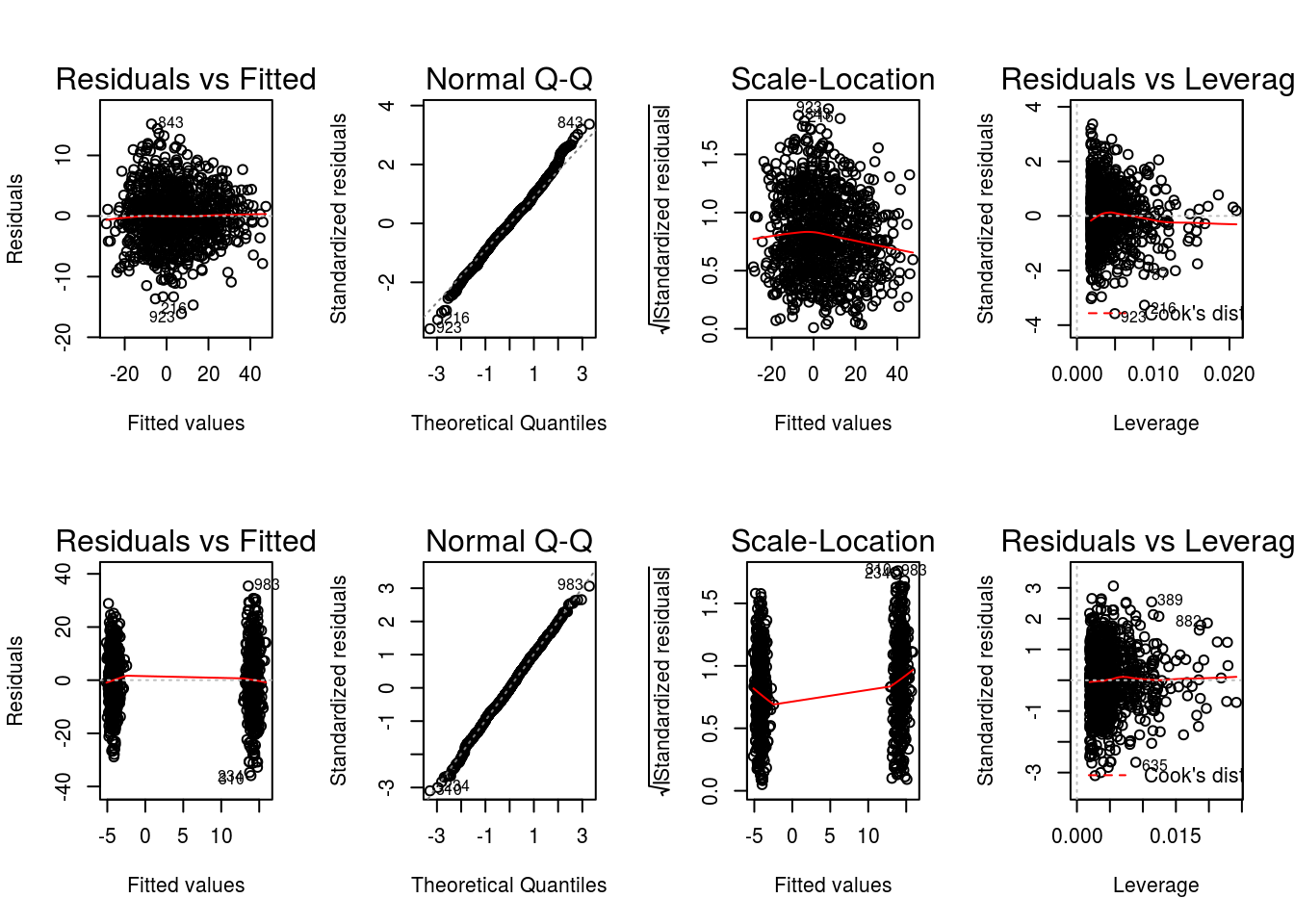
where we have included the diagnostic plots for model \(Q^{1}_{1}(h_{1},a_{1};\beta_{1})\) for easy comparison. We see that the residuals from the fit of model \(Q^{2}_{1}(h_{1},a_{1};\beta_{1})\) do not exhibit the two groupings, reflecting the fact that \(Q^{2}_{1}(h_{1},a_{1};\beta_{1})\) is only partially misspecified in that it includes the important covariate Ch.
Now, let’s examine the summary statistics for the regression step
summary(object = OR2)
Call:
lm(formula = YinternalY ~ Ch + A + Ch:A, data = data)
Residuals:
Min 1Q Median 3Q Max
-16.1012 -2.7476 -0.0032 2.6727 15.1825
Coefficients:
Estimate Std. Error t value Pr(>|t|)
(Intercept) 36.510110 0.933019 39.13 <2e-16 ***
Ch -0.205226 0.004606 -44.56 <2e-16 ***
A -89.524507 1.471905 -60.82 <2e-16 ***
Ch:A 0.507374 0.006818 74.42 <2e-16 ***
---
Signif. codes: 0 '***' 0.001 '**' 0.01 '*' 0.05 '.' 0.1 ' ' 1
Residual standard error: 4.511 on 996 degrees of freedom
Multiple R-squared: 0.907, Adjusted R-squared: 0.9068
F-statistic: 3239 on 3 and 996 DF, p-value: < 2.2e-16Comparing to the diagnostics for model \(Q^{1}_{1}(h_{1},a_{1};\beta_{1})\), we see that the residual standard error is smaller (4.51 vs 11.6) and that the adjusted R-squared value is larger (0.91 vs 0.38). Both of these results indicate that model \(Q^{2}_{1}(h_{1},a_{1};\beta_{1})\) is a more suitable model for \(E(Y|X=x,A=a)\) than model \(Q^{1}_{1}(h_{1},a_{1};\beta_{1})\).
The third model we will consider is the correctly specified model used to generate the dataset,
\[ Q^{3}_{1}(h_{1},a_{1};\beta_{1}) = \beta_{10} + \beta_{11} \text{Ch} + \beta_{12} \text{K} + a_{1}~(\beta_{13} + \beta_{14} \text{Ch} + \beta_{15} \text{K}). \]
Modeling Object
As for \(Q^{1}_{1}(h_{1},a_{1};\beta_{1})\) and \(Q^{2}_{1}(h_{1},a_{1};\beta_{1})\), the parameters of this model will be estimated using ordinary least squares via
The modeling object for this regression step is
q3 <- modelObj::buildModelObj(model = ~ (Ch + K)*A,
solver.method = 'lm',
predict.method = 'predict.lm')Model Diagnostics
For \(Q^{3}_{1}(h_{1},a_{1};\beta_{1})\) the regression can be completed as follows
OR3 <- modelObj::fit(object = q3, data = dataSBP, response = y)
OR3 <- modelObj::fitObject(object = OR3)
OR3
Call:
lm(formula = YinternalY ~ Ch + K + A + Ch:A + K:A, data = data)
Coefficients:
(Intercept) Ch K A Ch:A K:A
-15.6048 -0.2035 12.2849 -61.0979 0.5048 -6.6099 where for convenience we have made use of modelObj’s
Again, let’s start by examining the diagnostic plots defined for “lm” objects.
par(mfrow = c(2,4))
graphics::plot(x = OR3)
graphics::plot(x = OR2)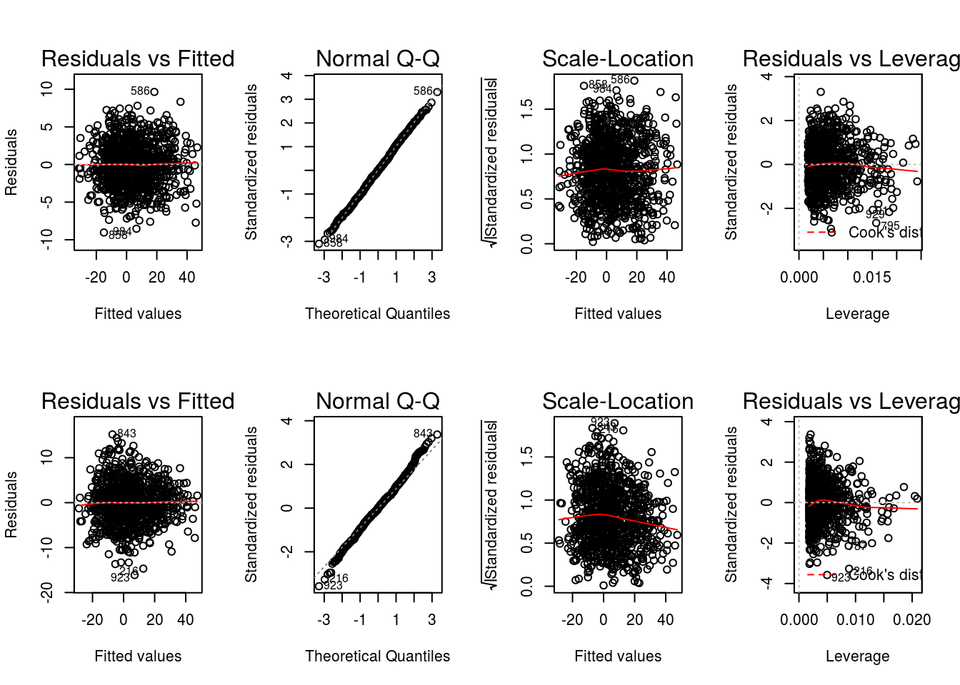
where we have included the diagnostic plots for model \(Q^{2}_{1}(h_{1},a_{1};\beta_{1})\) for easy comparison. We see that the results for models \(Q^{2}_{1}(h_{1},a_{1};\beta_{1})\) and \(Q^{3}_{1}(h_{1},a_{1};\beta_{1})\) are very similar, with model \(Q^{3}_{1}(h_{1},a_{1};\beta_{1})\) yielding slightly better diagnostics (e.g., smaller residuals); a result in line with the knowledge that \(Q^{3}_{1}(h_{1},a_{1};\beta_{1})\) is the model used to generate the data.
Now, let’s examine the summary statistics for the regression step
summary(object = OR3)
Call:
lm(formula = YinternalY ~ Ch + K + A + Ch:A + K:A, data = data)
Residuals:
Min 1Q Median 3Q Max
-9.0371 -1.9376 0.0051 2.0127 9.6452
Coefficients:
Estimate Std. Error t value Pr(>|t|)
(Intercept) -15.604845 1.636349 -9.536 <2e-16 ***
Ch -0.203472 0.002987 -68.116 <2e-16 ***
K 12.284852 0.358393 34.278 <2e-16 ***
A -61.097909 2.456637 -24.871 <2e-16 ***
Ch:A 0.504816 0.004422 114.168 <2e-16 ***
K:A -6.609876 0.538386 -12.277 <2e-16 ***
---
Signif. codes: 0 '***' 0.001 '**' 0.01 '*' 0.05 '.' 0.1 ' ' 1
Residual standard error: 2.925 on 994 degrees of freedom
Multiple R-squared: 0.961, Adjusted R-squared: 0.9608
F-statistic: 4897 on 5 and 994 DF, p-value: < 2.2e-16As for model \(Q^{2}_{1}(h_{1},a_{1};\beta_{1})\), we see that the residual standard error is smaller (2.93 vs 4.51) and that the adjusted R-squared value is larger (0.96 vs 0.91). Again, these results indicate that model \(Q^{3}_{1}(h_{1},a_{1};\beta_{1})\) is a more suitable model than both models \(Q^{1}_{1}(h_{1},a_{1};\beta_{1})\) and \(Q^{2}_{1}(h_{1},a_{1};\beta_{1})\).
\(\pi_{1}(h_{1};\gamma_{1})\)
Throughout Chapters 2-4, we consider three propensity score models selected to represent a range of model (mis)specification. Note that we are not demonstrating a definitive analysis that one might do in practice, in which the analyst would use all sorts of variable selection techniques, etc., to arrive at a posited model. Our objective is to illustrate how the methods work under a range of model (mis)specification.
Click on each tab below to see the model and basic model diagnostic steps. Note that this information was discussed previously in Chapter 2 and is repeated here for convenience.
The first model is a completely misspecified model having none of the covariates used in the data generating model
\[ \pi^{1}_{1}(h_{1};\gamma_{1}) = \frac{\exp(\gamma_{10} + \gamma_{11}~\text{W} + \gamma_{12}~\text{Cr})}{1+\exp(\gamma_{10} + \gamma_{11}~\text{W} + \gamma_{12}~\text{Cr})}. \]
Modeling Object
The parameters of this model will be estimated using maximum likelihood via
p1 <- modelObj::buildModelObj(model = ~ W + Cr,
solver.method = 'glm',
solver.args = list(family='binomial'),
predict.method = 'predict.glm',
predict.args = list(type='response'))Model Diagnostics
Though we will implement our treatment effect and value estimators in such a way that the regression step is performed internally, it is convenient to do model diagnostics separately here. We will make use of modelObj::
For \(\pi^{1}_{1}(h_{1};\gamma_{1})\) the regression can be completed as follows:
PS1 <- modelObj::fit(object = p1, data = dataSBP, response = dataSBP$A)
PS1 <- modelObj::fitObject(object = PS1)
PS1
Call: glm(formula = YinternalY ~ W + Cr, family = "binomial", data = data)
Coefficients:
(Intercept) W Cr
0.966434 -0.007919 -0.703766
Degrees of Freedom: 999 Total (i.e. Null); 997 Residual
Null Deviance: 1378
Residual Deviance: 1374 AIC: 1380where for convenience we have made use of modelObj’s
Now, let’s examine the regression results for the model under consideration.
summary(object = PS1)
Call:
glm(formula = YinternalY ~ W + Cr, family = "binomial", data = data)
Deviance Residuals:
Min 1Q Median 3Q Max
-1.239 -1.104 -1.027 1.248 1.443
Coefficients:
Estimate Std. Error z value Pr(>|z|)
(Intercept) 0.966434 0.624135 1.548 0.1215
W -0.007919 0.004731 -1.674 0.0942 .
Cr -0.703766 0.627430 -1.122 0.2620
---
Signif. codes: 0 '***' 0.001 '**' 0.01 '*' 0.05 '.' 0.1 ' ' 1
(Dispersion parameter for binomial family taken to be 1)
Null deviance: 1377.8 on 999 degrees of freedom
Residual deviance: 1373.8 on 997 degrees of freedom
AIC: 1379.8
Number of Fisher Scoring iterations: 4First, in comparing the null deviance (1377.8) and the residual deviance (1373.8), we see that including the independent variables does not significantly reduce the deviance. Thus, this model is not significantly better than the constant propensity score model. However, we know that the data mimics an observational study for which the propensity score is not constant or known. And, note that the Akaike Information Criterion (AIC) is large (1379.772). Though the AIC value alone does not tell us much about the quality of our model, we can compare this to other models to determine a relative quality.
The second model is an incomplete model having only one of the covariates of the true data generating model
\[ \pi^{2}_{1}(h_{1};\gamma_{1}) = \frac{\exp(\gamma_{10} + \gamma_{11} \text{Ch})}{1+\exp(\gamma_{10} + \gamma_{11} \text{Ch})}. \]
Modeling Object
As for \(\pi_{1}(h_{1};\gamma)\) the parameters of this model will be estimated using maximum likelihood via
The modeling objects for this regression step is
p2 <- modelObj::buildModelObj(model = ~ Ch,
solver.method = 'glm',
solver.args = list(family='binomial'),
predict.method = 'predict.glm',
predict.args = list(type='response'))The regression is completed as follows:
PS2 <- modelObj::fit(object = p2, data = dataSBP, response = dataSBP$A)
PS2 <- modelObj::fitObject(object = PS2)
PS2
Call: glm(formula = YinternalY ~ Ch, family = "binomial", data = data)
Coefficients:
(Intercept) Ch
-3.06279 0.01368
Degrees of Freedom: 999 Total (i.e. Null); 998 Residual
Null Deviance: 1378
Residual Deviance: 1298 AIC: 1302Again, we use
summary(PS2)
Call:
glm(formula = YinternalY ~ Ch, family = "binomial", data = data)
Deviance Residuals:
Min 1Q Median 3Q Max
-1.7497 -1.0573 -0.7433 1.1449 1.9316
Coefficients:
Estimate Std. Error z value Pr(>|z|)
(Intercept) -3.062786 0.348085 -8.799 <2e-16 ***
Ch 0.013683 0.001617 8.462 <2e-16 ***
---
Signif. codes: 0 '***' 0.001 '**' 0.01 '*' 0.05 '.' 0.1 ' ' 1
(Dispersion parameter for binomial family taken to be 1)
Null deviance: 1377.8 on 999 degrees of freedom
Residual deviance: 1298.2 on 998 degrees of freedom
AIC: 1302.2
Number of Fisher Scoring iterations: 4First, in comparing the null deviance (1377.8) and the residual deviance (1298.2), we see that including the independent variables leads to a smaller deviance than obtained from the intercept only model. And finally, we see that the AIC is large (1302.247), but it is less than that obtained for \(\pi^{1}_{1}(h_{1};\gamma_{1})\) (1379.772). This result is not unexpected as we know that the model is only partially misspecified.
The third model we will consider is the correctly specified model used to generate the data set,
\[ \pi^{3}_{1}(h_{1};\gamma_{1}) = \frac{\exp(\gamma_{10} + \gamma_{11}~\text{SBP0} + \gamma_{12}~\text{Ch})}{1+\exp(\gamma_{10} + \gamma_{11}~\text{SBP0}+ \gamma_{12}~\text{Ch})}. \]
The parameters of this model will be estimated using maximum likelihood via
The modeling objects for this regression step is
p3 <- modelObj::buildModelObj(model = ~ SBP0 + Ch,
                              solver.method = 'glm',
                              solver.args = list(family='binomial'),
                              predict.method = 'predict.glm',
predict.args = list(type='response'))The regression is completed as follows:
PS3 <- modelObj::fit(object = p3, data = dataSBP, response = dataSBP$A)
PS3 <- modelObj::fitObject(object = PS3)
PS3
Call:  glm(formula = YinternalY ~ SBP0 + Ch, family = "binomial", data = data)

Coefficients:
(Intercept)         SBP0           Ch
  -15.94153      0.07669      0.01589

Degrees of Freedom: 999 Total (i.e. Null);  997 Residual
Null Deviance:      1378
Residual Deviance: 1162 AIC: 1168Again, we use
summary(PS3)
Call:
glm(formula = YinternalY ~ SBP0 + Ch, family = "binomial", data = data)

Deviance Residuals:
    Min       1Q   Median       3Q      Max
-2.3891  -0.9502  -0.4940   0.9939   2.1427

Coefficients:
              Estimate Std. Error z value Pr(>|z|)
(Intercept) -15.941527   1.299952 -12.263   <2e-16 ***
SBP0          0.076687   0.007196  10.657   <2e-16 ***
Ch            0.015892   0.001753   9.066   <2e-16 ***
---
Signif. codes:  0 '***' 0.001 '**' 0.01 '*' 0.05 '.' 0.1 ' ' 1

(Dispersion parameter for binomial family taken to be 1)

    Null deviance: 1377.8  on 999  degrees of freedom
Residual deviance: 1161.6  on 997  degrees of freedom
AIC: 1167.6

Number of Fisher Scoring iterations: 3
First, we see from the null deviance (1377.8) and the residual deviance (1161.6) that including the independent variables does reduce the deviance as compared to the intercept only model. And finally, we see that the AIC is large (1167.621), but it is less than that obtained for both \(\pi^{1}_{1}(h_{1};\gamma_{1})\) (1379.772) and \(\pi^{2}_{1}(h_{1};\gamma_{1})\) (1302.247). This result is in-line with the knowledge that this is the data generating model.