Description
We compare the estimators introduced throughout Chapters 2-4 using a simulated data set that mimics a single decision point, observational study. The goal of this study is to assess the effectiveness of a fictitious medication developed for the treatment of hypertension (systolic blood pressure, SBP, greater than 140mmHg). The primary outcome of interest is the change in systolic blood pressure after six months of treatment.
The data set comprises one thousand patients (\(n=1000\)) diagnosed as hypertensive. Several baseline patient characteristics are available: SBP0, systolic blood pressure (mmHg); W, weight (kg); K, potassium level (mg/dl); Cr, creatinine level (mg/dl); and Ch, total cholesterol (mg/dl). Each patient in this study either received the new medication (\(A=1\)) or received no treatment (\(A=0\)) based on patient/physician discretion. Six months after the treatment decision, the systolic blood pressure of each patient was remeasured, SBP6. The observed data are independent and identically distributed
\[ \{\text{SBP0}_i, \text{W}_i, \text{K}_i, \text{Cr}_i, \text{Ch}_i, A_i, \text{SBP6}_i\},~ \text{for}~i = 1, \dots, n. \]
The primary outcome of interest is \(Y = \text{SBP}0-\text{SBP}6\), where larger values are considered better. We assume that all participants adhered to the treatment plan to which they were assigned and that no participants dropped out of the study.
For the simulation scenario used to generate the data, the true treatment effect is \(\delta^{\text{*}} = 17.4\). This scenario implies the following true outcome regression relationship
\[ Q_{1}(h_{1},a_{1}) = -15 - 0.2~ \text{Ch} + 12~ \text{K} + a_{1}~(-65 + 0.5~ \text{Ch} -5.5~ \text{K}), \]
and propensity
\[ \pi_{1}(h_{1}) = \frac{\exp(-16.348 + 0.0748~\text{SBP0} + 0.017~\text{Ch})}{1+\exp(-16.348 + 0.0748~\text{SBP0} + 0.017~\text{Ch})}. \]
The data generating models and the
Once downloaded, the data set can be loaded into R using
dataSBP <- utils::read.csv(file = 'path_to_file/hyper.txt', header = TRUE)where ‘path_to_file’ is the full path to the downloaded data set file.
Examining the first few records of the data set
utils::head(x = dataSBP) SBP0 W K Cr Ch A SBP6
1 148 101.2 3.7 0.6 167.7 0 154
2 164 50.3 4.4 0.9 174.4 0 161
3 164 70.6 3.7 0.7 202.2 1 160
4 164 65.8 4.1 1.0 297.2 0 191
5 173 84.4 3.5 0.8 242.6 1 155
6 165 66.5 3.6 0.9 254.7 1 145shows that our data set contains the expected covariates: SBP0, systolic blood pressure measured at baseline; W, weight; K, potassium level; Cr, creatinine level; Ch, total cholesterol; A the treatment received; and SBP6 systolic blood pressure measured six months post treatment.
We must define the outcome of interest, \(Y = \text{SBP}0-\text{SBP}6\), in the R environment.
y <- dataSBP$SBP0 - dataSBP$SBP6Note that larger values of the response are better; we seek to decrease patients’ systolic blood pressure.
Remark: \(y\) is referred to as ‘the response’ or ‘the outcome of interest’ interchangeably in
Simulation Scenario
The data for this simulated trial were generated from the following models:
set.seed(seed = 1234L)
n <- 1000L\[ \text{SBP0} \sim \mathcal{N}(\mu=160, \sigma^2=12^2) \]
and must satisfy the following constraint: \(140 \mathrm{mmHg} \lt \text{SBP}_{0} \le 200 \text{mmHg}\).
  # Probability that N(160,144) is below 140
  pSBP_L <- stats::pnorm(q = 140.0, mean = 160.0, sd = 12.0)

  # Probability that N(160,144) is below 200
  pSBP_U <- stats::pnorm(q = 200.0, mean = 160.0, sd = 12.0)

  # Generate uniform random values within these limits
  prob <- stats::runif(n = n, min = pSBP_L, max = pSBP_U)

  # Invert CDF to obtain SBP0
  SBP0 <- stats::qnorm(p = prob, mean = 160.0, sd = 12.0)
SBP0 <- round(x = SBP0, digit = 0L)Participants’ weights were obtained from height and body mass index, where height (H)
\[ \text{H} \sim \mathcal{N}(\mu=1.7, \sigma^2=0.1^2) \]
and body mass index (BMI)
\[ \text{BMI} \sim \mathcal{N}(\mu=25.0, \sigma^2=3.5^2); \]
\(\text{W} = \text{BMI}*\text{H}*\text{H}\).
  ## Generate weight

  # Generate n normally distributed heights
  height <- stats::rnorm(n = n, mean = 1.7, sd = 0.1)

  # Generate n normally distributed BMI values
  bmi <- stats::rnorm(n = n, mean = 25.0, sd = 3.5)

  # Calculate weight
  W <- bmi * height * height
W <- round(x = W, digit = 1L)\[ \text{K} \sim \mathcal{N}(\mu=4.2, \sigma^2=0.35^2). \]
  ## Generate potassium levels

  K <- stats::rnorm(n = n, mean = 4.2, sd = 0.35)
  K <- round(x = K, digit = 1L)
Creatinine levels where generated in a similar manner to \(\text{SBP0}\),where \(0.4 \le \text{Cr} \le 1.25\) and
\[ \text{Cr} \sim \mathcal{N}(\mu=0.82,\sigma^2=0.1^2). \]
  ## Generate Creatinine levels

  # Probability that N(0.82,0.01) is below 0.4
  pCr_L <- stats::pnorm(q = 0.4, mean = 0.82, sd = 0.1)

  # Probability that N(0.82,0.01) is below 1.25
  pCr_U <- stats::pnorm(q = 1.25, mean = 0.82, sd = 0.1)

  # Generate uniform random values within these limits
  prob <- stats::runif(n = n, min = pCr_L, max = pCr_U)

  # Invert CDF to obtain Cr
  Cr <- stats::qnorm(p = prob, mean = 0.82, sd = 0.1)
Cr <- round(x = Cr, digit = 1L)\[ \text{Ch} \sim \mathcal{N}(\mu=211, \sigma^2=45^2) \]
  ## Generate total cholosterol

  Ch <- stats::rnorm(n = n, mean = 211.0, sd = 45.0)
Ch <- round(x = Ch, digit = 1L)\[ A \sim B\{n=1, p= \pi_{1}(x_{1})\} \]
\[ \pi_{1}(x_{1}) = \text{expit}(-16.348 + 0.078~\text{SBP0} + 0.017~\text{Ch}) \] and \(\text{expit}(u) = e^{u}/(1+e^{u})\).
  ## Generate treatment variable

  probXB <- -16.348 + 0.078*SBP0 + 0.017*Ch
  prob <- exp(x = probXB) / (1.0 + exp(x = probXB))
A <- stats::rbinom(n = n, size = 1L, prob = prob)\[ \text{SBP6} = \text{SBP0} - \mathcal{N}(\mu=\mu_{SBP6},\sigma^2=3^2). \]
\[ \mu_{SBP6} = -15.0 - 0.2~\text{Ch} + 12.0~\text{K} + A (-65.0 + 0.5~\text{Ch} - 5.5~\text{K}) \]
  ## Generate change in Systolic Blood Pressure

  mn <- {-15.0 - 0.2*Ch + 12.0*K} + A*{-65.0 + 0.5*Ch - 5.5*K}
  y <- stats::rnorm(n = n, mean = mn, sd = 3.0)
  y <- round(x = y, digits = 0L)

  ## Systolic Blood Pressure at six months
  SBP6 <- SBP0 - y
The true treatment effect is \(\delta^{\text{*}} = -65.0 + 0.5*211 - 5.5*4.2 = 17.4\) mmHg.
Summary
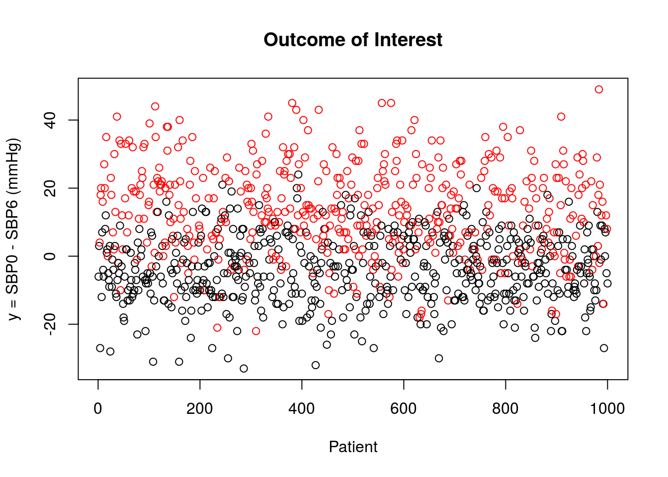
The outcome of interest, \(Y = \text{SBP0}-\text{SBP6}\), is plotted below for patients that did not receive treatment (black) and for those that received the new medication (red). Recall that we define the outcome of interest such that larger values are more desirable.

The summary data for each covariate is given below.
summary(object = dataSBP) SBP0 W K Cr Ch A SBP6
Min. :140.0 Min. : 37.50 Min. :3.10 Min. :0.5000 Min. : 83.0 Min. :0.000 Min. : 97.0
1st Qu.:153.0 1st Qu.: 63.30 1st Qu.:4.00 1st Qu.:0.8000 1st Qu.:178.8 1st Qu.:0.000 1st Qu.:146.0
Median :161.0 Median : 71.90 Median :4.20 Median :0.8000 Median :208.3 Median :0.000 Median :158.0
Mean :161.6 Mean : 72.65 Mean :4.21 Mean :0.8191 Mean :209.2 Mean :0.454 Mean :157.4
3rd Qu.:169.0 3rd Qu.: 80.90 3rd Qu.:4.40 3rd Qu.:0.9000 3rd Qu.:240.5 3rd Qu.:1.000 3rd Qu.:168.0
Max. :197.0 Max. :135.20 Max. :5.10 Max. :1.1000 Max. :332.4 Max. :1.000 Max. :214.0 
